1 INTRODUCTION
Gesture elicitation is widely used in Human-Computer Interaction (HCI) for identifying gesture vocabularies that are self-discoverable or easy to learn (Wobbrock et al. 2009). In a typical gesture elicitation study, participants are shown the outcome of user interface actions or commands and are asked to propose gestures that would trigger these actions. While the hope is that consistent gesture-to-action associations will emerge, participants may also not agree in their proposals. Thus, analyzing agreement between participants is a key aspect of the method (Vatavu and Wobbrock 2015, 2016; Wobbrock et al. 2009). Agreement analysis can guide the design of gesture vocabularies and help understand why some commands or actions naturally map to gestures.
A widely used measure for quantifying agreement in gesture elicitation studies is the index $A$ introduced by Wobbrock et al. (2005). The index has been recently superseded by a more accurate measure of agreement, the agreement rate $AR$ (Findlater et al. 2012; Vatavu and Wobbrock 2015). Vatavu and Wobbrock (2015) argued for the adoption of the new index and provided guidelines on how to interpret agreement rates by suggesting ranges of low, medium, high, and very high agreement. Furthermore, they proposed the $V_{rd}$ significance test for comparing agreement rates within participants. More recently, Vatavu and Wobbrock (2016) introduced the $V_b$ significance test for comparing agreement rates between independent groups of participants.
While statistics for analyzing agreement are important for gesture elicitation research, our article identifies three problems in the methods described by Vatavu and Wobbrock (2015, 2016):
- The $A$ and $AR$ indices do not take into account that agreement between participants can occur by chance. We demonstrate that chance agreement can be a problem even when gesture vocabularies are open-ended and participants choose from a large or infinite space of possible gestures. The reason is that agreement is often dominated by a small number of very frequent categories of gestures. We characterize this phenomenon as bias and model it with well-known probability distribution functions. We then evaluate its effect on chance agreement through Monte Carlo experiments.
- Guidelines for interpreting agreement rely on problematic assumptions about the probability distribution of $AR$ values and can lead to overoptimistic conclusions about the level of agreement reached by participants. We discuss additional reasons why the interpretation of agreement scores cannot be based on the methodology of Vatavu and Wobbrock (2015).
- The $V_{rd}$ and the $V_b$ statistics rely on probabilistic assumptions that yield extremely high Type I error rates. Our Monte Carlo experiments show that the average Type I error rate of both significance tests is higher than $40\%$ for a significance level of $\alpha =.05$. Our results contradict the evaluation results reported by Vatavu and Wobbrock (2016) for the $V_b$ statistical test.
These three problems can encourage an investigator to overestimate or misinterpret the agreement observed in a study or to conclude that there is agreement when in reality there is little or none. They can also cause the investigator to falsely assess random differences between agreement values as “statistically significant.” For example, we show that the conclusion of Vatavu and Wobbrock (2016) that women and men reach consensus over gestures in different ways, based on the dataset of Bailly et al. (2013), is not supported by statistical evidence.
We present solutions to these problems. These solutions build upon a vast literature on inter-rater reliability that has extensively studied how to assess agreement (Gwet 2014) and has advocated indices that correct for chance agreement. Chance-corrected indices, such as Cohen's $\kappa$, Fleiss’ $\kappa$, and Krippendorff's $\alpha$, are routinely used in a range of disciplines such as psychometrics, medical research, computational linguistics, as well as in HCI for content analysis, e.g., for video and user log analysis (Hailpern et al. 2009) or for the analysis of design outcomes (Bousseau et al. 2016). These indices allow us to isolate the effect of bias and understand how participants’ proposals differentiate among different commands. We also discuss criticisms of these indices and describe complementary agreement measures. The above literature has also established solid methods to support statistical inference with agreement indices. In this article, we advocate resampling techniques (Efron 1979; Quenouille 1949), which are versatile, easy to implement, and support both hypothesis testing and interval estimation. We conduct a series of Monte Carlo experiments to evaluate these methods.
We illustrate the use of chance-corrected agreement indices and interval estimation by re-analyzing and re-interpreting the results of four gesture elicitation studies published at CHI: a study of bend gestures (Lahey et al. 2011), a study of single-hand microgestures (SHMGs) (Chan et al. 2016), a study of on-skin gestures (Weigel et al. 2014), and a study of keyboard gestures (Bailly et al. 2013). Our analyses confirm that current methods regularly cause HCI researchers to misinterpret the agreement scores obtained from their studies and sometimes lead them to conclusions that are not supported by statistical evidence.
Previous work has recognized that HCI research often misuses statistics (Kaptein and Robertson 2012). This has prompted a call for more transparent statistics that focus on fair communication and scientific advancement rather than persuasion (Dragicevic 2016; Kay et al. 2016). Others have pointed to the lack of replication efforts in HCI research (Hornbæk et al. 2014; Wilson et al. 2012) and have urged the CHI community to establish methods that build on previous work, improve results, and accumulate scientific knowledge (Kostakos 2015). We hope that the critical stance we adopt in this article will contribute to a fruitful dialogue, encourage HCI researchers to question mainstream practices, and stress the need for our discipline to consolidate its research methods by drawing lessons from other scientific disciplines.
2 PRELIMINARIES
We start with background material that will later help us clarify our analysis. We introduce key concepts of gesture elicitation. We clarify the steps of the process and define our terminology. Finally, we introduce the main questions that we investigate in this article and summarize the overall structure of our analysis.
2.1 Referents, Gestures, and Signs
Many of the key concepts of gesture elicitation were introduced by Good et al. (1984), Nielsen et al. (2004), and Wobbrock et al. (2005, 2009). Wobbrock et al. (2009) summarize the approach as follows: participants are prompted with referents, or the effects of actions, and perform signs that cause those actions.
The analysis of Wobbrock et al. (2009) makes no distinction between gestures and signs. In our analysis, we distinguish between the physical gestures performed by participants and their signs. A sign can be thought of as the interpretation of an observed gesture, or otherwise, an identity “label” that provides meaning. A sign can also be considered as a category that groups together “equal” or “similar” gestures. For example, a “slide” sign can group together all sliding touch gestures, regardless of the number of fingers used to perform the gesture.
Classifying gestures into signs is rarely straightforward because their interpretation often relies on subjective human judgment. It also depends on the scope and the quality of the media used to record gestures, e.g., a video recording cannot capture a finger's force as the finger slides on a table. Data recording and interpretation issues are important for our analysis, as they largely affect agreement assessment. To account for data recording, we distinguish between the physical gesture and its recorded gesture description. To account for data interpretation, we then distinguish between the actual gesture elicitation study and the classification process, which takes place after the study and is responsible for classifying gesture descriptions into signs.
2.2 Gesture Elicitation and Data Collection
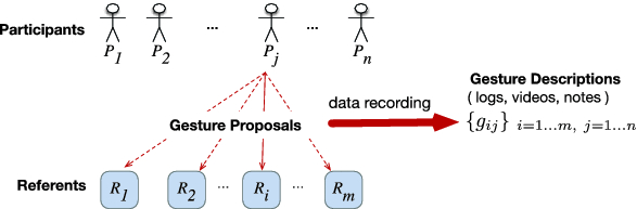
Figure 1 illustrates a gesture elicitation study, where $n$ participants ($P_1, P_2,\ldots,P_n$) propose (or perform) gestures for $m$ referents ($R_1, R_2,\ldots,R_m$). Gestures are recorded digitally, e.g., with a video camera and motion sensors, or manually, e.g., through questionnaires and observation notes. The output of a gesture elicitation study is a dataset $\lbrace g_{ij}\, | \, i=1..m, \, j=1..n\rbrace$ that describes all the proposed gestures, where $g_{ij}$ denotes the piece of data that describes the gesture proposed by participant $P_j$ for referent $R_i$. This dataset may combine diverse representations, such as log files, video recordings, and observation notes.
We take as an example a fictional scenario inspired by a real study (Wagner et al. 2012). Suppose a team of researchers seek a good gesture vocabulary for a future tablet device that senses user grasps. Their specific goal is to determine which grasp gestures naturally map to document navigation operations such as “scroll down” or “previous page.” To this end, they recruit $n=20$ participants to whom they show $m=10$ navigation operations, i.e., referents, in the form of animations on the tablet. Each participant is asked to propose a grasp gesture for each referent. Suppose data collection is exclusively based on video recordings that capture (i) how the participants perform the grasp gestures, and (ii) how they describe them by thinking aloud. The researchers collect a total of $20 \times 10 = 200$ grasp descriptions, where each grasp description consists of a distinct video recording. We use variations of this scenario to explain key issues throughout the article.
2.3 Gesture Classification Process and Sign Vocabularies
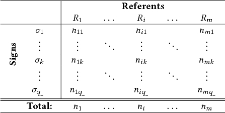
To analyze the findings of a gesture elicitation study, the researchers must first interpret their recorded gesture descriptions by classifying them into signs. Figure 2 illustrates a typical gesture classification process. We define this process as a function $C$ that takes as input a set of gesture descriptions $\lbrace g_{ij}\rbrace$ and produces a set of sign assignments $\lbrace g_{ij} \rightarrow \sigma _k\, |\, k=1..q_{\_}\rbrace$, such that each gesture description $g_{ij}$ is assigned a sign $\sigma _k$ that belongs to a sign vocabulary of size $q$. In the rest of the article, we make a distinction between $q$, which is the total number of possible signs, and $q_{\_} \le q$, which is the number of signs produced for a specific gesture elicitation study.
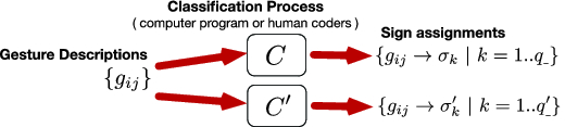
Gesture classification is most often performed by humans. However, for well-defined gestural alphabets such as EdgeWrite (Wobbrock et al. 2005), it can be automated and performed by a computer program. As shown in Figure 2, a different classification function $C^{\prime }$ will generally produce a different set of assignments over a different sign vocabulary. Gestures are often classified along multiple dimensions. For example, Weigel et al. (2014) classify on-skin gestures along two orthogonal dimensions: their on-body location (fingers, wrist, upper arm, etc.) and their input modality (pinch, twist, tap, etc.). Similarly, Bailly et al. (2013) classify separately the key and the gesture applied to the key of a Métamorphe keyboard. For other studies, gestures are grouped together into larger classes (Chan et al. 2016; Piumsomboon et al. 2013; Troiano et al. 2014) by considering a subset of gesture parameters. In this case, different grouping strategies result in different sign vocabularies.
In the simplest case, a sign vocabulary is defined through a set of discrete signs, where each sign maps to a unique combination of gesture parameters. In most cases, however, sign vocabularies are open-ended, i.e., they are not known or fixed in advance. Instead, they are defined indirectly through an identity or a similarity measure that determines whether any two gestures correspond to the same or two different signs. For example, Wobbrock et al. (2005, 2009) group “identical” (or “equal”) gestures together, while other approaches (Chan et al. 2016; Piumsomboon et al. 2013) have used less stringent criteria of gesture similarity.
As a consequence, the number of possible signs $q$ is often unknown. Thus, it can be claimed to be infinite ($q \rightarrow \infty$) such that given a similarity function, one can always find a gesture that is different (“unequal” or “not similar”) than all currently observed gestures. For example, one can trivially invent a new sign by taking the sequence of two existing signs. It could be argued that the assumption of an infinite sign vocabulary is artificial. However, it is an elegant abstraction that enables us to assess various agreement statistics in the more general case, when sign vocabularies are large, or at least larger than a small handful of 5–10 signs.
2.4 Agreement Assessment
Given a set of assignments of gesture descriptions to signs, one can check which signs are attributed to each referent and count their occurrences. Consider again our gesture elicitation study on grasp gestures. Suppose that a human coder reviews the video descriptions produced by the study – she inspects each video and classifies the proposed grasp gesture into a sign. Table 1 presents some fictitious results, where five unique signs (“A,” “B,” “C,” “D,” and “E”) are identified. For each referent (R1, R2 ... R10), the table shows the number of occurrences of each sign. Such tables are known as contingency tables and can be used to summarize the results of a gesture elicitation study to assess participants’ agreement. If a sign occurs more than once for a referent, we infer that at least two participants agree on this sign. Researchers usually seek signs that enjoy wide agreement among users. The larger the number of occurrences of a sign for a given referent, the greater is considered to be the evidence that the gesture is intuitive or a good match for that referent. Thus, agreement assessment has taken a key role in the analysis of gesture-elicitation results (Vatavu and Wobbrock 2015, 2016; Wobbrock et al. 2005, 2009).
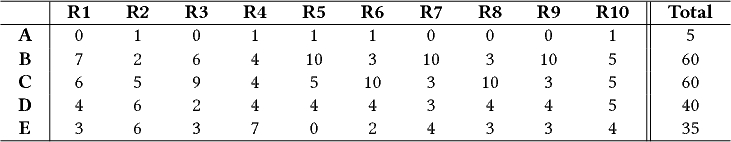 |
| Note: A total of 20 participants each propose a grasp gesture for 10 different referents (R1–R10). Each grasp gesture is classified into a sign: “A,” “B,” “C,” “D,” or “E.” Each cell shows the number of sign occurrences for a given referent. |
2.5 The Notion of Bias
Imagine that the five signs ($q_{\_}=5$) that emerged from our fictitious study is only a subset of a much larger sign vocabulary. In this case, how would one explain that fact that only these five signs appeared? Moreover, why are “B” and “C” so frequent (see Total in Table 1) while “A” is rare? We refer to this overall tendency of some signs to appear more frequently than others, independently of the actual referents, as bias.
Research in Linguistics and Cognitive Psychology has extensively studied the role of bias in the evolution and learning of both human and artificial languages. For example, Markman (1991) argues that young children acquire biases that help them rule out alternative hypotheses for the meaning of words and progressively induce the correct mappings between words and referents, such as objects and actions. Culbertson et al. (2012) characterize as bias universal constraints in language learning that shape the space of human grammars. Through experiments with artificial languages, they show that such biases are not simply due to external factors, such as historical or geographic influences, but instead, they are part of the learners’ cognitive system. In particular, they show that learners favor grammars with less variation (regularization bias) and prefer harmonic ordering patterns (harmonic bias) (Culbertson et al. 2012). Garrett and Johnson (2012) study the phonetic evolution of languages and identify a range of bias factors that cause certain phonetic patterns to appear more frequently than others: motor-planning processes, speech aerodynamic constraints, gestural mechanics, and speech perceptual constraints.
The role of such biases has not been fully understood in the context of gesture elicitation, but we can name several factors that may lead participants to focus on certain gestures or their properties and disregard others. Those include usability issues such as the conceptual, cognitive, and physical complexity of gestures, their discoverability, memorability, and so on. Considerations about the social acceptability of available gestures (Rico and Brewster 2010) can also shape participants’ choices. The effect of such biases is usually of great interest for a gesture elicitation study, as it can help researchers understand if certain gestures are more appropriate, e.g., easier to conceive, execute or socially accept, than others.
Other bias factors, however, can hamper the generalizability or the usefulness of gesture elicitation results. Morris et al. (2014) argue that “users’ gesture proposals are often biased by their experience with prior interfaces and technologies” and refer to this type of bias as legacy bias. According to the authors, legacy bias has some benefits (e.g., participants “draw upon culturally-shared metaphors”) and increases agreement scores but “limits the potential of user elicitation methodologies.” It is thus often considered that it hinders the novelty of the gestures produced by a gesture elicitation study.
The elicitation study procedure can also introduce bias. According to Ruiz and Vogel (2015), time-limited studies bias participants against considering long-term performance and fatigue. Other sources of procedural bias include the low fidelity of device prototypes presented to participants, which may prevent or reinforce the execution or detection of certain gestures, or the lack of clarity in investigators’ instructions. Finally, the classification of gesture proposals into signs can introduce additional bias. Gesture classification is often performed by the investigators, who also need to decide on how to differentiate among signs. This process usually relies on a mix of objective and subjective criteria, and thus investigators risk adding their own biases.
Usability, social, legacy, procedural, and classification biases are additive, so overall bias will be observed as an imbalance in the distribution of signs across all referents. This notion of bias has a central role in our analysis of agreement.
2.6 Questions and Structure of the Article
A gesture elicitation study can serve a range of design and research goals. The focus of this article is on questions that concern participants’ consensus on the choice of signs, where these questions mostly derive from earlier work by Wobbrock et al. (2005, 2009) and more recent work by Vatavu and Wobbrock (2015, 2016):
- Do participants agree on their gestures? Is their level of consensus high, either for individual referents or overall, for the full set of referents?
- How does agreement compare across different referents? Do some referents or groups of referents lead to lower or higher agreement?
- Do different groups of participants (e.g., novices vs. experts) demonstrate the same level of agreement? Does agreement vary across different user groups?
A visual inspection of the data in Table 1 reveals a mix of agreement and disagreement. Since some signs appear multiple times for many referents, one may argue that such patterns demonstrate agreement. However, given the uncertainty in the sample, is this agreement substantial or high enough to justify a user-defined vocabulary of gestures? Is it intrinsic or should it rather be attributed to chance? Furthermore, do all agreements have the same importance? For example, is not it easier to agree when the number of possible or obvious options is small? One may also try to compare agreement among different referents and conclude that agreement is higher for referents for which proposals are spread less uniformly (e.g., for R5), revealing one or a few “winning” signs. To what extent does statistical evidence support this conclusion? Do such patterns reveal real differences or are they random differences that naturally emerge by chance?
The above are all questions that we try to answer in this article. Specifically, we investigate the following three problems: (i) how to measure agreement (Sections 3 and 4), (ii) how to assess the magnitude of agreement (Section 5), and (iii) how to support statistical inference over agreement measures (Section 6). For each of these three problems, we review existing solutions, focusing on recent statistical methods introduced by Vatavu and Wobbrock (2015, 2016). We identify a series of problems in these methods. Inspired by related work in the context of inter-rater reliability studies (see Gwet's (2014) handbook for an overview of this work), we introduce alternative statistical methods, which we then use to reanalyze the results of four gesture elicitation studies (Section 7). A key argument of our analysis is that any kind of bias can deceive researchers about how participants agree on signs. The agreement measures that we recommend remove the effect of bias. We show how researchers can investigate bias separately with more appropriate statistical tools.
We explained that participants do not directly propose signs. However, in certain sections (Sections 5 and 6), we will write that participants “propose” and “agree on their signs” or refer to “participants’ sign proposals.” Although these expressions do not accurately describe how participants’ proposals are assigned to signs, they simplify our presentation without impairing the validity of our analysis.
3 MEASURING AGREEMENT
To quantify agreement over a referent $R_i$, a great number of elicitation studies have used the formula of Wobbrock et al. (2005):
 |
Later on, Findlater et al. (2012) refine $A_i$ with a slightly different index, which can be written as follows:
It is worth noting that neither $AR_i$ nor its approximation $A_i$ are new. They have been used in a range of disciplines as measures of homogeneity for nominal data. They have been independently reinvented several times in the history of science (Ellerman 2010) and are most commonly referred to as the Simpson's (1949) index. The $AR$ index is also well known and is commonly referred to as the percent agreement (Gwet 2014). However, it is also widely known to be problematic, as we will now explain.
3.1 The Problem of Chance Agreement
Consider again our fictitious study of grasp gestures. The overall agreement rate $AR = .265$ can be valued as respectable, as it is slightly higher than the average $AR$ reported by Vatavu and Wobbrock (2015) from 18 gesture elicitation studies. According to their recommendations, it can be interpreted as a medium level of agreement.
However, the researchers have reasons to be worried. Suppose the study is replicated, but participants are now blindfolded and cannot see any of the referents presented to them – they are simply asked to guess. Their grasp proposals will thus be random. Suppose the researchers follow the same gesture classification process, classifying gestures into five signs ($q=5$). If all five signs are equally likely, they will all appear with a probability of $1 / 5= .2$. Thus, the probability that any pair of participants “agree” on the same sign is $.2 \times .2$. Since two participants can agree on any of the five signs, the probability of agreement for a pair of participants on any given referent is $5 \times .2 \times .2 = .2$. Therefore, the expected proportion of participant pairs who are in agreement – that is, the expected overall agreement rate $AR$ – is $.2$.
Surprisingly, this value is not far from the previously observed value ($AR = .265$) and can be interpreted again as medium agreement (Vatavu and Wobbrock 2015). However, given that there is no intrinsic agreement between participants, one would rather expect an agreement index to give a result close to zero. Furthermore, one would certainly not label such a result as a “medium” agreement. We should note that the exact same result would emerge if participants were not blindfolded but, instead, the gesture classification process was fully random.
Arguably, the blindfolded study is purely fictional, and no gesture elicitation study involves participants who make completely random decisions. Nevertheless, gesture elicitation involves subjective judgments, where randomness can play a role. A participant may be uncertain about which gesture is the best, and in some situations, the participant may even respond randomly. Such situations may arise as a result of highly abstract referents for which there is no intuitive gesture, poor experimental instructions, gesture options that are too similar, or a lack of user familiarity with the specific domain or context of use. Due to sources of randomness in participants’ choice of gestures, any value of $AR$ reflects both intrinsic and spurious agreement. The amount of spurious agreement depends on the likelihood of chance agreement, which in turn depends on the number of signs.
The vocabulary of five signs used in our example is rather small. One could argue that if participants choose from a large space of possible signs, then chance agreement would be practically zero. However, a large space of possible signs does not eliminate the problem of chance agreement. We will next show that bias can greatly increase the likelihood of chance agreement and inflate agreement rates even if the size of a sign vocabulary is large or infinite ($q\rightarrow \infty$).
3.2 Modeling Bias and Showing its Effect on Chance Agreement
We first illustrate the problem of bias with a scenario from a different domain. Suppose two medical doctors independently evaluate the incidents of death of hospitalized patients. For each case, they assess the cause of each patient's death by using the classification scheme of the World Health Organization,1 which includes 132 death cause categories. Suppose information about some patients is incomplete or missing. For these cases, the two doctors make uncertain assessments or simply try to guess. How probable is it that their assessments agree by chance?
If one assumes that the doctors equally choose among all 132 categories, the probability of agreement by chance is negligible, as low as $1/132 = .76\%$. However, the assumption of equiprobable categories is not realistic in this case. Most death causes are extremely rare, while the two most common causes, the ischemic heart disease and the stroke, are alone responsible for more of $25\%$ of all deaths. The 10 most frequent ones are responsible for more than $54\%$ of all deaths.2 It is not unreasonable to assume that uncertain assessments of the two doctors will be biased toward the most frequent diseases. In this case, the problem of chance agreement can be serious, as results that appear as agreement on frequent categories may hide uncertain or even random assessments.
In the above example, the source of bias is prior knowledge about the frequency of diseases, where in the absence of enough information, doctors tend to minimize the risk of a false diagnosis by favoring frequent over rare diseases. In gesture elicitation, bias has other sources – we have already discussed them in Section 2. To understand how bias affects chance agreement, we mathematically describe it as a monotonically-decreasing probability-distribution function $b(k)$, $k=1, 2,..\infty$, where the bias function gives the probability of selecting the $k{\text{th}}$ most probable sign when ignoring or having no information about the referent. The function is assumed to be asymptotically decreasing such that $b(k) \rightarrow 0$ when $k \rightarrow \infty$.
We focus on two well-known probability distributions that have the above properties: (i) the discrete half-normal distribution, and (ii) the Zipf–Mandelbrot distribution (Mandelbrot 1967). The first is the discrete version of the well-known normal (Gaussian) distribution when we only consider its right half. We set its mean to $k=1$ and control the bias level by varying the standard deviation $sd$ (see Figure 3(b)). The distribution converges to uniform (bias disappears) as $sd \rightarrow \infty$.
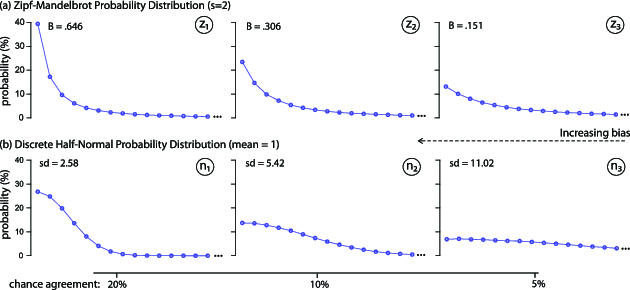
The second is a generalization of Zipf's (1949) law and is widely used in computational linguistics to model word frequencies in text corpora. Zipfian distributions occur for a diverge range of phenomena (Newman 2005). They have also applications in HCI, as several studies have shown that they are good models for predicting the frequency of command use (Cockburn et al. 2007). The original explanation given by Zipf (1949) for his law was based on the principle of least effort, according to which the distribution of word use is due to a tendency to communicate efficiently with least effort. Mandelbrot (1967), in turn, argued that such distributions may arise from minimizing information-theoretic notions of cost. Although several other generative mechanisms have been proposed, the theoretical explanation of Zipf's law is still an open research problem (Newman 2005). Interestingly, an early experiment by Piantadosi (2014) shows that Zipfian distributions can even occur for completely novel words, whose frequency of use could not be explained by any optimization mechanism of language change. According to the author, a possible explanation of the law is its link with power-law phenomena in human cognition and memory (Piantadosi 2014).
While the Zipf law has a single parameter $s$, the Zipf–Mandelbrot distribution has two parameters $s$ and $B$, where the latter allows us to control for bias:
The two distribution functions are not the only possible alternatives. Nevertheless, they have very distinct shapes and allow us to experimentally demonstrate the effect of bias on agreement under two different model assumptions. Notice that we can generate an infinite range of intermediate probability functions by taking a linear combination of the two base functions: $b(k)=\alpha b_{zipf}(k)+(1-\alpha)b_{normal}(k)$, where $\alpha \in [0..1]$. Finally, we can trivially use the same distributions to describe noninfinite sign vocabularies by constraining their tails, i.e., by setting $b(k)=0$ for $k\gt q$.
Experiment 3.1. We demonstrate how bias increases chance agreement with a Monte Carlo experiment implemented in R. The experiment simulates the situation where participants make fully random proposals under bias. More specifically, we consider that 20 blindfolded participants are presented 40 different referents, and for each referent, they are asked to propose a gesture. Participants’ gestures are then classified into signs, where the number of possible signs is infinite. We test all the six bias distributions presented in Figure 3. For each, we take 5,000 random samples, and each time we calculate $AR$. The mean value of $AR$ can be considered as an estimate of chance agreement, since any agreements occur by chance – participants cannot see any referents presented to them.
The experiment results in chance agreement scores that are very close to the ones presented in Figure 3: (i) $20\%$ for the bias distributions $z_1$ and $n_1$, (ii) $10\%$ for the bias distributions $z_2$ and $n_2$, and (iii) $5\%$ for the bias distributions $z_3$ and $n_3$. Such levels of chance agreement are not negligible. They are also realistic, as we later demonstrate in Section 7. The mean number of unique signs $q_\_$ that we observed in our experiment is as follows:
 |
Not surprisingly, higher bias leads to smaller sign vocabularies. Notice that the Zipf–Mandelbrot distribution clearly leads to a larger number of signs. This is an expected result because Zipfian distributions are well known to have long tails, i.e., a large portion of occurrences far from the distribution's head.
3.3 Chance-Corrected Agreement
A large volume of research has examined the issue of chance agreement in the context of inter-rater reliability studies, i.e., studies that involve subjective human assessments (Gwet 2014). Such assessments are made in studies that involve qualitative human judgments, such as classifying patients into disease categories, interpreting medical images, annotating speech, or coding open survey responses. If reliability is of concern, typically two or more people (raters) are asked to perform the same judgments, and their agreement is used as a proxy for reliability.
Inter-rater reliability studies employ a different terminology from gesture elicitation studies, but the mapping between the two is straightforward. Study participants become raters (also called judges or coders), referents become items (also called subjects), and signs become categories (Gwet 2014).
Work on chance-corrected agreement dates back to the 50–60s. Early on, Cohen (1960) proposed the $\kappa$ (Kappa) coefficient to measure the agreement between two raters:
Note that $\kappa$ can take negative values: while a positive value means agreement beyond chance, a negative value means disagreement beyond chance – although this rarely happens in practice. Also note that if $p_a = 1$, then $\kappa =1$ (provided that $p_e \ne 1$). Thus, chance correction does not penalize perfect agreement.
Most chance-corrected agreement indices known today are based on Equation (4). Each index makes different assumptions and has different limitations (Gwet 2014). Early indices such as Cohen's (1960) $\kappa$ and Scott's (1955) $\pi$ assume two raters. As gesture elicitation involves more participants, we will not discuss them further. A widely used index that extends Scott's $\pi$ to multiple raters is Fleiss’ (1971) $\kappa _F$ coefficient. For the term $p_a$ in Equation (4), Fleiss uses the “proportion of agreeing pairs out of all the possible pairs of assignments” (Fleiss 1971), also called percent agreement. This formulation for $p_a$ has been used in many other indices and is identical to the $AR$ index of Vatavu and Wobbrock (2015).
For the chance agreement term $p_e$, Fleiss uses
In gesture elicitation, raters’ (i.e., participants’) proposals are classified into categories (i.e., signs) after the end of the study by a separate gesture-classification process. The interpretation of chance agreement now changes because chance agreement also captures the additional bias of this higher-level classification process (see Section 2.5). Notice that sign vocabularies can be open-ended. However, this open-endedness does not affect how Fleiss’ $\kappa _F$ coefficient is computed because the coefficient requires no prior knowledge or assumption about the number of possible signs $q$. Equations (2) and (5) only depend on the number of observed signs $q_{\_}$ and their frequencies.
An alternative index is the $\kappa _q$ coefficient of Brennan and Prediger (1981), which uses the same $p_a$ but a simpler estimate of chance agreement: $p_e = 1/q$, where $q$ is the total number of categories. The index assumes equiprobable selection of categories. Under this assumption, the chance agreement for Table 1 is $p_e = .200$, and thus $\kappa _q = .081$. However, as we explained earlier, this assumption is generally not realistic, as it does not account for bias. The index has been further criticized for giving researchers the incentive to add spurious categories in order to artificially inflate agreement (Artstein and Poesio 2008). If one assumes an infinite number of categories, then $p_e = 0$. For all these reasons, the index is rarely used in practice.
Another measure of agreement, widely used in content analysis, is Krippendorff's $\alpha$ (Krippendorff 2013). Krippendorff's $\alpha$ uses a different formulation for both $p_a$ and $p_e$ and can be used for studies with any number of raters, incomplete data (i.e., not all raters rate all items), and different scales including nominal, ordinal and ratio. For simple designs, its results are generally very close to Fleiss’ $\kappa _F$, especially when there are no missing data and the number of raters is greater than five (Gwet 2014). We use both indices in our analyses with a preference for Fleiss’ $\kappa _F$, as it is simpler and easier to contrast to the $AR$ index.
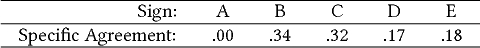
Experiment 3.2. We repeat the Monte Carlo experiment presented in Section 3.2, but this time, we also calculate Fleiss’ chance agreement $p_e$, Fleiss’ $\kappa _F$, and Krippendorff's $\alpha$. Mean estimates for each bias distribution (see Figure 3) are presented below:
 |
We see that Fleiss’ $p_e$ provides a very good estimate of chance agreement for all six distributions. Thus, it can be considered as a good measure for assessing the effect of bias on agreement, even if one assumes an infinite number of signs. Both Fleiss’ $\kappa _F$ and Krippendorff's $\alpha$ completely remove the effect of bias, returning consistent agreement scores that are very close to zero. We have repeated the experiment with other bias distributions, e.g., by taking the linear combination of the above distributions with variable weights. Again, results were the same.
The above chance-corrected coefficients do not only work on average. For the 30,000 iterations (6 distributions $\times$ 5,000 iterations) of our experiment, Fleiss’ $\kappa _F$ ranged from $\kappa _{F,min}=-.018$ to $\kappa _{F,max}=.019$, while Krippendorff's $\alpha$ ranged from $\alpha _{min}=-.017$ to $\alpha _{max}=.020$, which means that the full range of chance-corrected scores was very close to zero. We expect the spread of values to increase for experiments with a smaller number of participants ($n\lt20$) or a smaller number of referents ($m\lt40$).
3.4 Agreement over Individual or Groups of Referents
So far, we have discussed how to correct overall agreement scores. In gesture elicitation studies, researchers are often interested in finer details concerning agreement, i.e., situations in which agreement is high and situations that exhibit little consensus. To this end, the analysis of agreement scores for individual items (i.e., referents) is a useful and commonly employed method. The state-of-the art approach in HCI is to use Equation (2), but unfortunately, this method does not account for chance agreement.
Research on inter-rater agreement has mostly focused on the use of overall agreement scores, but agreement indices for individual items also exist. For example, O'Connell and Dobson (1984) introduced an agreement index that can be computed on an item-per-item basis, and Posner et al. (1990) further explained its calculation. For the most practical cases that we study here, the index is identical to Fleiss’ $\kappa _F$ calculated for individual items, using a pooled $p_e$. Specifically, one can compute $p_a$ for each referent of interest and then use Equation (5) to estimate a common $p_e$ across all referents. The rationale is that, by definition, chance agreement does not depend on any particular referent. The same method can be employed for assessing agreement over groups of referents.
We apply the approach to the data in Table 1. The observed percent agreement for R5 is $p_a=.321$, and the overall chance agreement is $p_e=.251$, computed over all referents of the study (see Equation (5)). Thus, Fleiss’ chance-corrected agreement for this referent is $\kappa _{F,5} = \frac{.321 - .251}{1 - .251} = .094$. For R10, the agreement is $\kappa _{F,10} = \frac{.190 - .251}{1 - .251} = -.082$. This negative value may suggest disagreement.
3.5 Is Correction for Chance Agreement Always Necessary?
Chance correction is a monotonically decreasing function that scales and offsets all per-referent $p_a$ scores but preserves their order. Thus, if only ordinal information is of interest (e.g., which are the most and the least consensual referents within a single study?), the use of standard agreement rates ($AR_i$) as in Equation (2) is acceptable. Similarly, if two different groups share the same chance agreement $p_e$, using $AR$ to compare their difference in agreement is a valid approach. The reason is that $\Delta p_a = p_{a,1} - p_{a,2}$ scales $\Delta \kappa = \kappa _1 - \kappa _2$ by a fixed amount ($1-p_e$) without distorting the underlying distribution (see Equation (4)). So the results of such comparisons should also generalize to $\kappa$. Section 6 further discusses this point.
There is a last question to answer. Bias is not necessarily harmful. In particular, it may be largely due to considerations about the effectiveness or cognitive complexity of different signs, irrespective of the referent to which these signs apply. Thus, bias may reflect participants’ overall agreement about which signs are appropriate candidates for a future gesture vocabulary. Since understanding such bias may be crucial, one could argue that chance-corrected coefficients like Fleiss’ $\kappa _F$ or Krippendorff's $\alpha$ are not appropriate in this case.
We agree that the analysis of bias is important. However, we argue that bias should be studied separately. We present three main reasons:
- Researchers need to know how participants distinguish among referents and whether natural mappings between signs and referents emerge. In the presence of any source of bias, the $AR$ index provides misleading information about how participants agree or disagree on their sign assignments.
- The bias distribution can be easily derived from the overall distribution of sign frequencies. This distribution is enough to fully describe bias and reveals which signs are frequent and which signs are absent or rare. Therefore, the reasoning behind translating a bias distribution into an agreement score is unclear. However, if investigators still want to quantify bias as agreement, a possible measure for this purpose is Fleiss’ chance agreement $p_e$, which can be reported in addition to $\kappa$.
- Distinguishing between different bias factors may not be feasible so the interpretation of an $AR$ score can be extremely problematic. Participants’ proposals are often dominated by obvious or “default” signs, e.g., the “top” sign in the study by Bailly et al. (2013), or signs that represent common gestures in widespread interfaces, e.g., multitouch gestures in the study by Weigel et al. (2014). Bias does not only concern participants’ original proposals. As we discussed, their classification is also subject to bias, and $AR$ gives investigators the incentive to invent frequent signs to artificially inflate agreement scores.
For all these reasons, correcting for chance agreement is important. However, given that chance-corrected coefficients have received multiple criticisms (see next section) and the HCI community has not yet arrived to a consensus, we advice authors to report both chance-corrected and uncorrected agreement values. Reporting both values increases transparency and can help researchers to better interpret their results. A separate investigation of the observed bias distribution is also recommended for every gesture elicitation study.
4 CRITICISMS OF CHANCE-CORRECTED AGREEMENT INDICES
Chance-corrected agreement coefficients are the norm in inter-rater reliability studies but have also received criticism. We address two types of criticism: (i) questioning the appropriateness of chance correction for gesture elicitation, and (ii) arguing that chance correction can lead to “paradoxically” low and unstable values for $\kappa$. After responding to these criticisms, we discuss some complimentary agreement measures.
4.1 Criticism 1: Chance Correction Is Not Appropriate for Gesture Elicitation
In a previous report, we recommended the use of chance-corrected agreement indices in addition to or as a replacement of the $AR$ index (Tsandilas and Dragicevic 2016). Vatavu and Wobbrock (2016) included a short discussion about this issue, where they argued that chance-corrected agreement indices are not appropriate for gesture elicitation studies:
“Unfortunately, the above statistics are not appropriate to evaluate agreement for elicitation studies, during which participants suggest proposals for referents without being offered any set of predefined categories. The particularity of an elicitation study is that the researcher wants to understand participants’ unconstrained preferences over some task, which ultimately leads to revealing participants’ conceptual models for that task. Consequently, the range of proposals is potentially infinite, only limited by participants’ power of imagination and creativity.” [pp. 3391–3392]
Gesture elicitation studies have certainly unique features. We agree that most gestures elicitation studies do not enforce a fixed set of sign categories. However, as we already discussed, the problem of chance agreement is still present. The argumentation of Vatavu and Wobbrock (2016) overlooks some key points:
- Kappa coefficients do not require choosing from a predefined set of categories. The a-posteriori classification of items to categories is not unique to gesture elicitation. For example, medical doctors do not use predefined classification schemes for diagnosis. They usually write open-ended reports or notes. Later, medical coders translate these reports into medical codes (O'Malley et al. 2005). Assessing agreement between diagnosis methods often requires medical experts with diverse roles to make assessments at multiple steps. For example, psychiatric clinicians prepare a brief psychiatric narrative of each case, and those narratives are reviewed by independent psychiatrists, who then classify the cases into diagnosis categories (Deep-Soboslay et al. 2005). As with gesture elicitation, the classification of cases into diagnosis categories only happens at the very end of the process and is not performed by the actual clinicians who evaluate the patients. A $\kappa$ coefficient is again computed over those top-level categories (Deep-Soboslay et al. 2005).
- Sign vocabularies can be limited. In practice, agreement is not assessed over an infinite set of gesture possibilities. Participants’ gesture proposals are first classified into signs (see Section 2), and agreement is assessed over the sign vocabulary defined by that specific classification process. We show in Section 7 that a sign vocabulary can be limited because investigators may use a particularly small number of signs to classify proposals.
- Proposals are often biased toward a small number of signs. Even if one assumes an infinite number of signs, chance agreement is still a problem due to various sources of bias that result in uneven distributions of sign frequencies. A major strength of Fleiss’ $\kappa _F$ (and Krippendorff's $\alpha$) is the fact that it corrects for bias by estimating chance agreement based on the distribution of observed signs. By taking into account this distribution, chance-corrected indices reward variability in participants’ proposals and highlight methodological problems.
Chance-corrected indices are the norm in content analysis where data are often open-ended and coders choose from codebooks that contain a large number of codes. According to MacQueen et al. (1998), “coders can reasonably handle 30–40 codes at one time,” while coding with codebooks of “more than 40 codes” is common, but the coding process needs to be done in stages. In computational linguistics, vocabularies can be even larger. In their coder's manual, Jurafsky et al. (1997) report on language modeling projects involving as many as 220 unique coding tags, where these tags are later clustered under 42 larger classes. Despite the use of such large vocabularies in these domains, chance agreement is always taken seriously, because codes typically do not occur with the same frequency, and coders are often biased toward a small subset of the coding vocabulary.
Arguably, chance agreement does not equally concern all gesture elicitation studies. The issue can be minor or nonexistent if three conditions are met: (i) participants choose from a large space of gestures, (ii) their proposals discriminate between many of these gestures with low bias, and (iii) the gesture classification process differentiates between subtle gesture variations. Nevertheless, the decision of whether chance correction is needed is best not to be left to the subjective discretion of each researcher – it is safer to always report chance-corrected agreement indices in addition to raw agreement rates (percent agreement). As their use is a well-established practice in many disciplines, there is no reason why gesture elicitation studies cannot benefit from them.
4.2 Criticism 2: Chance Correction Can Lead to Paradoxes
Chance-corrected coefficients such as Cohen's and Fleiss’ $\kappa$ penalize imbalanced distributions, where some categories are frequent while others are rare. Feinstein and Cicchetti (1990) argue that this can lead to “paradoxes,” where (i) $\kappa$ can be particularly low despite the fact that the observed percent agreement $p_a$ is high, and (ii) $\kappa$ can be very sensitive to small changes in the distribution of marginal totals.
We demonstrate their argument with two fictional datasets (see Table 3), where three participants propose signs for 10 referents. Participants are almost in full agreement for Dataset 1, and percent agreement is $p_a=.93$. However, Fleiss applies a high chance correction $p_e = .76$, which results in $\kappa _F =.72$. Dataset 2 is almost identical to Dataset 1, where the only difference is P3’s proposal for R7. Percent agreement has only slightly dropped ($p_a=.87$), but Fleiss’ $\kappa _F$ has dropped radically ($\kappa _F =.28$). Why is $\kappa _F$ so low even if data suggest high consensus among participants? Furthermore, why does a small change cause $\kappa _F$ to drop so radically?
| R1 | R2 | R3 | R4 | R5 | R6 | R7 | R8 | R9 | R10 | ||
| Dataset 1 | P1 | A | A | A | A | A | A | B | A | A | A |
| P2 | A | A | A | A | A | A | B | A | A | A | |
| P3 | A | A | A | A | A | A | B | C | A | A | |
| Dataset 2 | P1 | A | A | A | A | A | A | B | A | A | A |
| P2 | A | A | A | A | A | A | B | A | A | A | |
| P3 | A | A | A | A | A | A | A | C | A | A | |
| Note: Three participants (P1, P2, P3) propose signs for 10 different referents (R1–R10). The only difference between the two datasets is P3’s proposal for R7. |
|||||||||||
Feinstein and Cicchetti (1990) explain that the source of such paradoxes is the assumption of $\kappa$ coefficients that raters are biased, i.e., they have a “relatively fixed prior probability” of making responses. Referring to their experience in clinical research, the authors argue that there is no reason to assume that such prior (bias) probabilities are established in advance. They complain that penalizing observed imbalances as evidence of prior bias, and thus chance agreement may not be fair. The way $\kappa$ coefficients estimate chance agreement has been criticized by other authors (Gwet 2014; Uebersax 2015) for very similar reasons.
Kraemer et al. (2002) reject the argument that these situations indicate a flaw of $\kappa$ or a paradox. In response to the above criticism, they argue that “it is difficult to make clear distinctions” between cases when “those distinctions are very rare or fine. In such populations, noise quickly overwhelms the signals.”
Consider a different scenario where two medical tests are evaluated for the diagnosis of HIV. Suppose the two tests highly agree (>98$\%$) on negative results (i.e., HIV is not present) but demonstrate zero agreement on positive results (i.e., HIV is present). Given the rareness of positive results (e.g., $1\%$ of all cases), percent agreement will be extremely high. However, a high agreement score is misleading, since the two tests completely fail to agree on the presence of HIV. In contrast, Fleiss’ (or Cohen's) $\kappa$ would be low in this case, since chance agreement is high. In most cases, this is a desirable behavior rather than a drawback of $\kappa$ coefficients. Whether the two tests make a deliberate choice when assessing negative cases or whether they make a random choice, the high chance correction applied by $\kappa$ is justified by the fact that such results are practically not meaningful and cannot be trusted. As Kraemer et al. (2002) explain, a “$\kappa = 0$ indicates either that the heterogeneity of the patients in the population is not well detected by the raters or ratings, or that the patients in the population are homogeneous.”
Krippendorff (2011) further discusses the above issues. He explains that in such scenarios, percent agreement is high but “uninformative” due to the “lack of variability.” In our example in Table 3, participants have used only three signs, and the “A” sign has highly dominated their preferences. The fact that they agree on “A” is not informative, as there is very little evidence about consensus on other signs. The higher Fleiss’ $\kappa _F$ that we found for Dataset 1 can be explained by a perfect consensus on “B,” in addition to a high consensus on “A.” In Dataset 2, consensus on “B” decreases while signs other than “A” become extremely rare, causing Fleiss’ $\kappa _F$ to radically drop.
Krippendorff (2011) discusses that chance-corrected agreement indices are more sensitive to rare than to frequent cases. However, the high sensitivity that we observe in our example is due to the low number of samples. Using three or two raters is common in inter-rater reliability studies but very unlikely in the context of gesture elicitation studies, where the number of participants is typically greater than 10. Furthermore, we argue later that agreement values should not be reported alone. Interval estimates can capture and communicate the uncertainty or sensitivity of estimated chance-corrected agreement values.
To increase the amount of information of a study, Krippendorff (2011) suggests that researchers should try to ensure variability. To paraphrase his statement, unless there is evidence for participants (coders) to have exercised their ability to distinguish among signs (units), “the data they generate are meaningless” (Krippendorff 2011). In such cases, a high percent agreement can be very misleading, while a low $\kappa$ must always alarm researchers. For example, did participants focus on a very small set of signs? Did the researchers in the above example tend to classify proposals as “A” to artificially inflate agreement? A strong bias toward obvious or “default” signs, inadequate instructions (e.g., ones that would encourage participants to explore a larger variety of gestures), bias in the gesture classification process, or a poorly chosen design space are all possible problems, where each requires a different treatment.
Ensuring variability is especially important for designing rich and meaningful gesture vocabularies. Therefore, establishing measures that encourage variability has very practical design implications. We further argue that $\kappa$ coefficients are especially appropriate for the analysis of gesture elicitation results, since the presence of a prior bias probability is a very realistic assumption (see Sections 2.5 and 3.2). Assuming that participants equally choose among an infinite number of possible signs by only considering the individual properties of each referent is a naive approach that, in several situations, could result in suboptimal design solutions.
4.3 Alternative Measures: Agreement Specific to Categories
Others have argued that a single agreement score cannot fully describe how raters agree with each other (Cicchetti and Feinstein 1990; Spitzer and Fleiss 1974; Uebersax 2015). Consider again the scenario of the two HIV diagnosis tests. Instead of a single measure of agreement, two separate measures could be used: (i) a measure specific to positive and (ii) a measure specific to negative test results. In this case, the investigators would aim for high agreement for both result categories. The advantage of the approach is that one can distinguish between high agreement for one category, e.g., negative test results, and low agreement for the other, e.g., positive test results. The approach is analogous to the use of sensitivity, otherwise recall, and specificity measures for the evaluation of binary classification tasks. Cicchetti and Feinstein (1990) recommended using these two indices in conjunction with chance-corrected agreement, viewing the approach as a remedy to the paradoxes of $\kappa$ coefficients.
To deal with multiple agreement categories, which is our focus here, Uebersax (1982) describes a more generic formulation of agreement specific to categories, or specific agreement:
 |
We observe that specific agreement is higher for the two frequent signs (“B” and “C”). It is zero for “A,” which appears rarely and with no consensus among participants.
Specific agreement can be used as a complementary measure, as it helps investigators to identify where low or high agreement occurs. However, its interpretation for more than two categories is not straightforward. As a general principle, observing high agreement over a few very frequent signs may indicate a low overall agreement. Spitzer and Fleiss (1974) further argued that specific agreement itself should be corrected for chance agreement. If the bias distribution is common across all participants, the proportion of chance agreement specific to a sign $k$ is given by the term $\pi _k$ in Equation (5) (Uebersax 1982). This term represents the occurrence frequency of that sign across all participants and all referents. Then, we can use Equation (4) to derive the proportion of chance-corrected agreement specific to each individual sign. For the previous example, results are as follows:
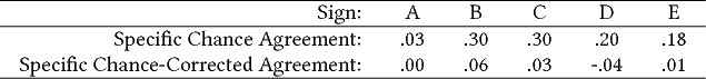 |
After chance correction, specific agreement is close to zero for all four signs.
For our analyses in Section 7, we report raw, i.e., without chance correction, specific agreement. Nevertheless, our interpretation also considers the observed frequencies of signs. Krippendorff (2011) has proposed additional information measures as companions of chance-corrected coefficients, but we will not discuss them in this article.
5 INTERPRETING THE MAGNITUDE OF AGREEMENT
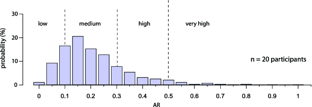
How much agreement is sufficient for a vocabulary of user-defined gestures? What criteria can investigators use to differentiate between low and high consensus? In response to these questions, Vatavu and Wobbrock (2015) have proposed some generic guidelines on how to interpret the magnitude of agreement: $AR \lt .100$ is low agreement, $.100 \lt AR \lt .300$ is medium, $.300 \lt AR \lt .500$ is high, and $AR \gt .500$ is very high agreement. These guidelines derive from two types of analysis: (i) a probabilistic reasoning, and (ii) a survey of agreement rates from past gesture elicitation studies.
In this section, we review the above guidelines. Our analysis indicates that both the probabilistic reasoning and the survey of past studies can lead to incorrect conclusions. We examine how other disciplines interpret agreement values and discuss the implication of these practices for gesture elicitation studies.
5.1 Probabilistic Reasoning
Vatavu and Wobbrock (2015) present an analytical approach to derive the probability distribution of agreement rates ($AR$) and use this distribution to identify the low, medium, and high range of probable agreement rates (see Figure 4). They then use these ranges to interpret the magnitude of observed agreement rates. For example, they estimate that the probability of obtaining an agreement rate $AR\gt.500$ is less than $1\%$, so they interpret observed agreement rates of this magnitude as very high. In contrast, they interpret agreement rates near the middle range of the probability distribution as medium agreement.
We identify two flaws in this reasoning:
- Flaw 1. It relies on a null distribution, i.e., a probability distribution of agreement rates by assuming completely random proposals. Yet, the authors’ analysis overlooks this fact and handles the null distribution as a distribution of observed agreement rates under no assumption of how agreement between participants takes place. Given the use of a null distribution, the derived interpretation guidelines are absurd. For example, the average of their distribution is $\overline{AR} = .214$ for $n=20$ participants and $\overline{AR} = .159$ for $n=40$ participants. Values close to these averages are interpreted as medium agreement despite the fact that they correspond to fully random proposals. According to the authors, values in the interval of medium agreement ($.100 - .300$) occur (simply by chance) with a $59\%$ probability. Wouldn't it make more sense to look for agreement (low, medium, or high) away from these ranges? Shouldn't we rather interpret values in these ranges as “no agreement?”
- Flaw 2. To derive the probability distribution, Vatavu and Wobbrock (2015) enumerate all possible partitions of integer $n$, where $n$ is the total number of participants. According to this solution, each partition represents a distinct configuration of sign proposals. For example, suppose we partition six participants into four groups with one, one, two, and two participants each: $1 + 1 + 2 + 2 = 6$. In this case, there are four distinct signs, and there is one agreement (i.e., two participants propose the same sign) for two of these signs. The authors assume that all such partitions occur with the exact same probability. For example, for a study with six participants (see Table 4), they assume that the probability that all six participants agree (partition $t_{11}$: 6) is equal to the probability that participants completely disagree (partition $t_{1}$: $1 + 1+ 1+ 1+ 1+ 1$) or only agree in pairs (partition $t_8$: $2 + 2 + 2$).
Unfortunately, this assumption is incorrect for two reasons. First, the number of alternative ways to assign participants to each partition is not the same. As shown in Table 4, there are $f_8=15$ different ways to partition six participants into pairs, but there is only $f_{11}=1$ way to create a single group of six. As a result, the two partitions $t_8$ and $t_{11}$ must occur with very different probabilities. We see later that the analysis of Vatavu and Wobbrock (2016) for their $V_b$ statistic corrects this mistake.
Second, agreement and disagreement do not generally occur with the same probability. For example, full agreement ($t_{11}$: 6) is very unlikely to occur when participants randomly choose from a very large set of possible signs. Full disagreement ($t_1$: $1+1+1+1+1+1$) is far more likely to occur in this case. The authors’ later analysis for the $V_b$ statistic repeats this second mistake.
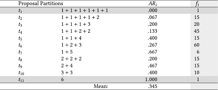 |
| Note: For six participants, they identify 11 possible partitions $t_i$ and assume that they all occur with the same probability. Under this assumption, the mean agreement rate (of random proposals) is calculated by averaging the individual agreement rates $AR_i$. Problem: Assuming equiprobable partitions is incorrect for two reasons: (i) The number $f_i$ of alternative ways to create each partition is not the same, e.g., $f_6 = 60 \times f_1$. Thus, partitions do not all occur with the same frequency. (ii) Agreement and disagreement do not occur with the same probability. For example, full agreement ($t_{11}$) and full disagreement ($t_1$) cannot occur with the same probability unless chance agreement is exactly $50\%$, e.g., if participants choose between two only signs with no bias. |
Can we correct the above mistakes and still rely on a probabilistic reasoning to interpret the magnitude of agreement rates? To answer this question, we first need to infer the correct null distribution of agreements. This is not feasible unless we know how participants choose signs. Analytical solutions to this problem are not trivial. Fortunately, such distributions can be approximated with Monte Carlo simulations. Specifically, we simulate a gesture elicitation study as a computerized process, where $n$ participants randomly propose signs for $m$ referents. This process is repeated a large number of times, and each time, a new agreement score is computed.
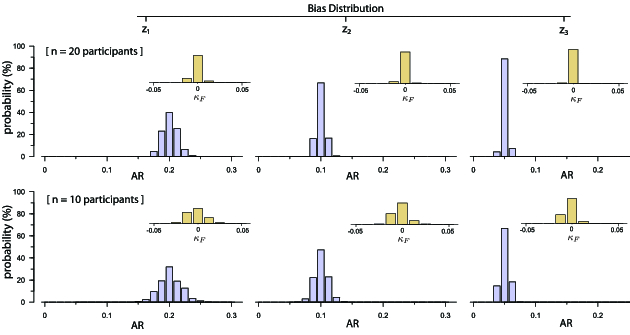
As in Section 3.2, we assume that participants choose from an infinite number of signs under bias. Figure 5 shows six distributions for two sample sizes ($n = 10$ and $n = 20$) and three bias levels. Here, we use the Zipf–Mandelbrot distribution to model bias (see Figure 3), but one can run Monte Carlo simulations with other prior bias-distribution assumptions. In all cases, the mean agreement rate approximates the chance agreement $p_e$, and the larger the number of participants, the more likely it becomes to find agreement rates close to $p_e$. In orange, Figure 5 presents the distributions of Fleiss’ $\kappa _F$. As expected, all these distributions are centered around zero.
Given such distributions, one can visually assess if an observed agreement value is likely to have occurred by chance. The further the value from the null distribution, the greater are the chances that agreement is different than zero. Such distributions are commonly known as sampling distributions of a statistic and serve as the basis for constructing confidence intervals and significance tests (Baguley 2012). However, they say very little about the magnitude of agreement, i.e., whether an observed agreement value is low, medium, or high. Unfortunately, this is a more complex problem that solutions based on probabilities and statistics cannot address.
5.2 Survey of Past Studies
In addition to their probabilistic reasoning, Vatavu and Wobbrock (2015) review agreement rates from a total of 15 papers with gesture elicitation results. They find that average $A$ scores range from .160 to .468, while average $AR$ scores range from .108 to .430, where the mean value is .261. They rely on these results to further justify their guidelines.
However, comparing agreement rates across different studies can be misleading because chance agreement can be high for some studies and low for others (see Section 3). We further show in Section 7 that a higher $AR$ score does not always translate into a higher chance-corrected agreement. The approach is problematic for additional reasons. Setting standards based on results from past studies seems a reasonable approach, but it can discourage efforts to raise our standards. Indeed, there does not seem to be any valid reason to be satisfied with a gesture agreement rate of .2 or .4.
Gwet (2014) dedicates a full chapter on how to interpret the magnitude of an agreement. Several authors suggest conventional thresholds to help researchers in this task – Fleiss, for example, labels $\kappa \lt .400$ as “poor” and $\kappa \gt .750$ as “excellent.” Krippendorff (2004) suggests $\alpha \gt .667$ and then later $\alpha \gt .800$ as thresholds below which data must be rejected as unreliable. However, he and many others recognize that such thresholds are largely arbitrary and should be chosen depending on the application domain and on the “costs of drawing invalid conclusions from these data” (Krippendorff 2004). It has also been emphasized that the magnitude of an agreement cannot be interpreted if confidence intervals are not provided (Gwet 2014; Krippendorff 2004).
In gesture elicitation studies, the bar for an agreement score to be considered acceptable is way lower, even when ignoring chance agreement. As much as we would like to have objective rules to help us distinguish between acceptable and unacceptable agreement scores, it is wise to refrain from using any such rule until these can be grounded in cost-benefit analyses that integrate usability metrics.
6 STATISTICAL INFERENCE
Statistical inference is the process of drawing conclusions about populations by observing random samples. It includes deriving estimates and testing hypotheses. Vatavu and Wobbrock (2015, 2016) have proposed two statistical tests to support hypothesis testing: (i) the $V_{rd}$ statistic for comparing agreement rates within participants (Vatavu and Wobbrock 2015), and (ii) the $V_{b}$ statistic for comparing agreement rates between independent participant groups (Vatavu and Wobbrock 2016).
We explained earlier (see Section 3.5) that comparing raw agreement rates is a valid approach as long as chance agreement is common across all compared groups. For within-participants designs, this is a valid assumption. In contrast, when comparing independent participant groups, chance agreement may vary, particularly when making comparisons across studies that test different sign vocabularies or employ different setups. Nevertheless, if groups are tested under similar conditions, and their data are analyzed with identical methods, there is no reason to expect bias differences. In this case, one can assume that chance agreement is equal for both groups, and therefore comparing agreement rates with the $V_{b}$ statistic could be considered as valid. However, we show that both the $V_{rd}$ and the $V_{b}$ statistic are based on incorrect probabilistic assumptions, and therefore they should not be used.
6.1 Modeling Agreement for Individual Referents
Before we examine the significance tests of Vatavu and Wobbrock (2015, 2016), we explore probabilistic models that describe how participants’ sign proposals to reach agreement for individual referents. As with bias, modeling agreement for individual referents will enable us to systematically evaluate the significance tests through Monte Carlo experiments.
Suppose that $n$ participants propose signs for $m$ referents, and let $AR_i$ be the agreement rate for referent $R_i$. We model sign preferences for this referent as a monotonically-decreasing probability-distribution function $p_i(k)$, $k=1, 2, ...\infty$, which expresses the probability of selecting the $k{\text{th}}$ most likely sign for referent $R_i$. Note that each referent $R_i$ will generally have its own distribution $p_i$, and the order of preferences over signs may also be different. The distribution function is assumed to be asymptotically decreasing such that $p_i(k) \rightarrow 0$ when $k \rightarrow \infty$. Clearly, the closer the distribution function to uniform is, i.e., no preferences over particular signs emerge, the lower is expected to be an observed agreement rate $AR_i$.
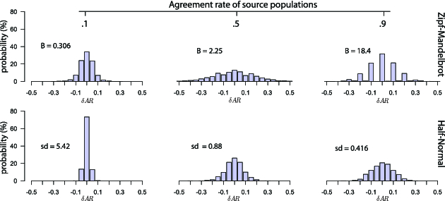
The above formulation is very similar to our bias formulation in Section 3.2. As for bias, we simplify our analysis by focusing on two probability distribution functions: (i) the discrete half-normal distribution with $mean = 1$, and (ii) the Zipf–Mandelbrot distribution with $s=2$. Given these distributions, one can generate source populations with a specific $AR_i$ by varying their parameters $sd$ or $B$. For example, for the half-normal distribution function, we choose $sd=5.42$ for $AR_i=.1$, $sd=.88$ for $AR_i=.5$, and $sd=.416$ for $AR_i=.9$. For the Zipf–Mandelbrot distribution function, we choose $B=.306$ for $AR_i=.1$, $B=2.25$ for $AR_i=.5$, and $B=18.4$ for $AR_i=.9$.
Significance tests focus on differences between agreement rates rather than individual agreement rates. Figure 6 shows the sampling distribution ($n = 20$) of the difference in agreement ($\delta AR = AR_i - AR_j$) between two referents $R_i$ and $R_j$, when sign preferences for those referents follow the same probability distribution, and $\delta AR = 0$. We examine six different distributions of sign preferences, which produce sampling distributions for three agreement levels: .1, .5, and .9. Notice that the spread of the sampling distribution is narrower for the half-normal distribution. It becomes especially narrow, when the agreement level of the source population is low ($AR_i=.1$).
6.2 The $V_{rd}$ Statistic: Testing Within-Participants Effects
The $V_{rd}$ statistic (Vatavu and Wobbrock 2015) can be used to compare agreement rates of different referents (or groups of referents) and test hypotheses such as (i) “there is an effect of the referent type on agreement” or (ii) “participants demonstrate higher agreement for directional than non-directional referents.”
The test is a direct application of Cochran's (1950) Q nonparametric test, which is used to test differences on a dichotomous dependent variable (with values coded as 0 or 1) among $\mu$ related groups.4 Cochran's Q test is analogous to the one-way repeated-measures ANOVA but for a dichotomous rather than a continuous dependent variable. For example, one can test whether there are differences in student performance ($1 =$ pass or $0 =$ fail) among three different courses (e.g., Mathematics, Physics, and Chemistry). A key assumption of Cochran's Q test is that cases, such as students in the above example, are randomly sampled from a population, and thus they are all independent.
In order to apply Cochran's Q test, Vatavu and Wobbrock (2015) enumerate all the possible pairs of participants and handle pairs as independent cases (see Table 5). Then, they consider agreement as a dichotomous variable that can take two values: 1 for agreement or 0 for disagreement. Given this approach, applying Cochran's Q test is straightforward, since the goal is to test differences in agreement among $\mu$ referents, or otherwise, $\mu$ related groups.
 |
| Note: Participant pairs $(P_i, P_j)$ are handled as independent cases, which are randomly sampled from a population of participant pairs. For six participants, there is a total of 15 participant pairs. Agreement observations are represented by binary values, where participants either agree (1) or disagree (0). |
Unfortunately, this solution is problematic because agreement pairs are highly interdependent, which is against the independence assumption of Cochran's Q test. For example, if participant $P_a$ agrees both with participant $P_b$ and participant $P_c$, we can safely deduce that participants $P_b$ and $P_c$ agree with each other. Similarly, if $P_a$ agrees with participant $P_b$ but disagrees with participant $P_c$, then we can deduce that participants $P_b$ and $P_c$ disagree. By assuming that agreement pairs are independent cases, the solution artificially increases the number of independent observations: $\mu \times n$ independent observations from $n$ participants are transformed to $\mu \times \frac{n(n-1)}{2}$ observations. For the six participants of our example, Figure 7 explains how to infer agreement for all 15 participant pairs from 5 only observations.
As this approach greatly overestimates the statistical power of the significance test, one can predict that the test is too sensitive to observations of random differences, or it rejects the null hypothesis too often. We demonstrate the problem with two Monte Carlo experiments that estimate the Type I error rate of the $V_{rd}$ test.
Experiment 6.1. We reimplemented the $V_{rd}$ statistic by using the implementation of Cochran's Q test in coin’s (Hothorn et al. 2008) statistical package for R. Our implementation accurately reproduces the values reported by Vatavu and Wobbrock (2015) for the study of Bailly et al. (2013). This confirms that our implementation is correct.
Our simulation experiment is as follows. We repeatedly generate $n$ random samples of proposals for $\mu =2$ referents, where $n$ represents the number of participants in a gesture elicitation study. We repeat the process by taking samples from nine source populations, where each approximates a different agreement rate $AR$, from .10 to .90. To generate populations for each $AR$ level, we use either the Zipf–Mandelbrot or the discrete half-normal probability distribution, as explained in Section 6.1.
We estimate Type I error rates for two significance levels: $\alpha =.05$ and $\alpha =.01$. For each source population, we run a total of $1,600$ iterations, where each time, we generate two random samples of size $n$. Given that these two samples are randomly generated from the same population, the percentage of iterations where the statistical test rejects the null hypothesis provides an estimate of its Type I error rate. Type I error rates should be close to $5\%$ for $\alpha = .05$ and close to $1\%$ for $\alpha = .01$. We test $n=20$, which is a typical size for gesture elicitation studies.
Table 6 summarizes our results. All error rates are extremely higher than their nominal values, reaching an average of $40\%$ to $60\%$ for the Zipf–Mandelbrot distributions. For the discrete half-normal distributions, error rates are lower but still unacceptably high. We can easily explain the lower error rates that we observe in this case by considering the narrower spread of the corresponding sampling distributions in Figure 6. One can test the $V_{rd}$ statistic with other prior distributions, e.g., by taking linear combinations of our two model distributions. Type I error rates will be within the above ranges of error, where the discrete half-normal distribution serves as a lower bound.
 |
| Note: The test is applied over randomly generated proposals of 20 participants for $\mu =2$ referents (1,600 iterations). The source population of sign proposals follows either a Zipf–Mandelbrot or a discrete half-normal distribution that approximates the target agreement rate: $AR = .10,$ .20,….90. |
Experiment 6.2. The second experiment is similar to the first, but we now use real data from Bailly et al. (2013) to generate populations from which we draw random samples. Bailly et al. (2013) elicited gestures applied to the keys of a keyboard from 20 participants for a total of 42 referents. We use the sign distribution within each referent to create a large population of $\hbox{6,000}$ sign proposals by random sampling with replacement. This process produces a total of 42 populations with agreement rates, ranging from $AR=.12$ to $AR=.91$ ($median =.32$). Then, for each population, we repeatedly generate $n=20$ random samples of proposals for $\mu =2$ referents. As before, we apply the $V_{rd}$ statistic to test whether the difference between their agreement rates is statistically significant.
After $1,600$ iterations, we find the following Type I error rates:
 |
These results are consistent with the results of Experiment 6.1. Error rates are extremely high for all tested populations.
6.3 The $V_b$ Statistic: Comparing Agreement between Independent Participant Groups
The $V_b$ statistic (Vatavu and Wobbrock 2016) can be used to compare agreement rates of independent participant groups and test hypotheses such as (i) “women demonstrate higher agreement than men” or (ii) “touch gestures receive higher agreement than full-body gestures on referents that represent navigation actions.” Previous work (Vanbelle and Albert 2009) has developed agreement indices to evaluate agreement between independent rater groups, but these indices answer a different type of questions, such as “do women agree with men?” Since such questions are out of the scope of the $V_b$ statistic, we do not discuss them here.
Vatavu and Wobbrock (2016) are inspired by Fisher's (1954) exact test to construct their test, but this time, they develop their own probabilistic framework to account for dependencies among participant pairs (see Figure 7). Their reasoning is similar to the one they previously used (Vatavu and Wobbrock 2015) to derive the probability distribution of $AR_i$ values (see Section 5.1). They generate all possible proposal partitions $t_i$ and estimate their probabilities $\pi _i$ (see Table 7). Then, they use these partial probabilities to estimate the overall probability of agreement. Here, we focus on how the authors derive the probabilities $\pi _i$ of individual partitions. For further details about the full test construction, we refer the reader to its original presentation by Vatavu and Wobbrock (2016).
 |
| Note: For seven participants, there are 15 possible partitions, where each partition $t_i$ appears with a different frequency $f_i$. Each probability $\pi _i$ is calculated by dividing $f_i$ by all 877 possible proposal configurations. Each partition $t_i$ corresponds to a different number $a_i$ of agreeing pairs. Problem: We highlight the two extreme cases in purple: full agreement ($t_{15}$) and full disagreement ($t_1$). Their probabilities are always assumed as equal ($\pi _{15}=\pi _1$), unfortunately, this assumption is not justified. |
As discussed in Section 5 (see Table 4), different partitions do not generally appear with the same frequency $f_i$. Table 7 shows how Vatavu and Wobbrock (2016) calculate the probability $\pi _i$ of all 15 possible partitions for seven participants, where frequencies $f_i$ are now taken into account. However, this solution still does not consider how difficult or how easy it is to reach agreement. For example, it relies again on the assumption that full agreement (i.e., all participants propose the same sign) and full disagreement (i.e., each participant proposes a different sign) always occur with the same probability. This assumption is unfortunately not realistic.
The authors’ own evaluation of the $V_b$ statistic demonstrate extremely low Type I error rates for $AR \ge .200$. As shown in Table 8 (gray columns), Vatavu and Wobbrock (2016) report error rates that are orders of magnitude lower than their nominal significance levels. Such error rates are problematic, and one could suspect that the test is too conservative. Nevertheless, the authors also present results from a number of case studies, where the $V_b$ test is shown to be powerful enough to reject the null hypothesis for many comparisons of practical interest. To clarify this issue, we re-evaluated the Type I error rate of the test with two simulation experiments.
 |
| Note: The significance test is applied on two independent groups of 20 participants for 1,600 iterations. The source population of sign proposals follows either a Zipf–Mandelbrot or a discrete half-normal distribution that approximates the target agreement rate: $AR = .10,$ .20,….90. Estimations of Type I error rates reported by Vatavu and Wobbrock (2016) (copied from page 3396) are shown in gray. |
Experiment 6.3. We reimplemented the $V_b$ statistic and the authors’ original algorithm that derives the probability distribution for two independent participant groups. Our implementation accurately reproduces p-values reported by Vatavu and Wobbrock (2016) for their case studies, which confirms that our implementation is correct.5 Our simulation method is similar to the one reported by the authors. We repeatedly generate populations of 100 participants, from which we draw two samples of equal size (20 participants each). We repeat this process for nine populations, where each population approximates a different agreement rate, from .10 to .90.
Vatavu and Wobbrock (2016) do not explain how they generate populations with controlled agreement rates, so we use again the Zipf–Mandelbrot and the discrete half-normal probability distribution functions. For each, we run a total of $1,600$ iterations and estimate the Type I error rate for two significance levels: $\alpha =.05$ and $\alpha =.01$.
Table 8 summarizes our evaluation results. Type I error rates are again extremely high for both distribution functions. Surprisingly, with the exception of $AR = .10$, our estimations are orders of magnitude higher than the ones reported by Vatavu and Wobbrock (2016) (see gray columns).
Experiment 6.4. As for Experiment 6.2, we use the dataset of Bailly et al. (2013) to generate populations, from which we draw random samples. We first generate a large population of $\hbox{6,000}$ users by random sampling with replacement from the sign proposals of the 20 participants of the original study. This process produces a total of 42 referent populations with agreement rates ranging from $AR = .12$ to $AR = .91$ ($median = .33$). We then repeatedly sample from this population to create two groups of 20 participants, and each time, we apply the $V_{b}$ statistic to test whether the agreement rates of the two independent groups are different for each of the 42 referents.
After $1,600$ iterations, we find the following Type I error rates:
 |
Results are consistent with the results of Experiment 6.3. Error rates are again unacceptably high for nearly all tested populations – only 2 out of 42 referent populations lead to Type I error rates that are close to their nominal levels.
6.4 Alternative Inference Methods: Jackknifing and Bootstrapping
Inventing new statistics can be dangerous, as the HCI community lacks the expertise to validate them and check their correctness. Other research disciplines have long established methods to support statistical inference for agreement indices (Gwet 2014; Hayes and Krippendorff 2007; Wood 2005). These are the methods that we present in this section.
The sampling distribution of an agreement index can be hard to approximate with analytical methods. However, resampling methods such as jackknifing (Quenouille 1949) and bootstrapping (Efron 1979) can be used to produce variance estimates, standard errors, and confidence intervals for almost any agreement index, including agreement rates, $\kappa$ coefficients, and agreement specific to categories. Confidence intervals can be used both to communicate uncertainty and to test hypotheses (Dragicevic 2016). We show how to use such methods to (i) provide an interval estimate of an agreement score, (ii) compare agreement between two groups of referents, and (iii) compare agreement between two independent participant groups.
6.4.1 Estimating Agreement Scores. To draw samples, it is crucial to first determine what is randomly sampled and what is not. In gesture elicitation studies, referents are fixed: any conclusion typically only applies to these referents. Participants, in contrast, are chosen randomly, and investigators may need to generalize their conclusions to the entire population of potential users. Gwet (2014) explains how to use the jackknife method to derive estimates of agreement indices in such situations, when raters are randomly chosen, while rated items are fixed.
Given observations from $n$ participants, estimation is based on $n$ subsamples, where each time, a subsample $i$ is produced by leaving out all the observations from the $i{\text{th}}$ participant. The confidence interval of an agreement index $\kappa$ is constructed by first estimating the variance of its sampling distribution:
Assuming that $\kappa$ coefficients follow a normal distribution, the $(1-\alpha)\%$ confidence interval is $\hat{\kappa } \pm SE_{jack} \times q$, where $q = q(1 - \frac{\alpha }{2}, n - 1)$ is the $(1 - \frac{\alpha }{2})$-quantile of Student's t-distribution with $n-1$ degrees of freedom. Gwet (2008) shows that normality is a reasonable assumption as long as the number of raters (i.e., participants) and items (i.e., referents) are reasonable high, and the agreement score is not close to its boundary values. Our evaluation further examines this assumption.
6.4.2 Comparing Agreement Scores of Related Samples. The same technique can be used to compare agreement scores obtained from the same participants between different groups of referents, i.e., for within-participants estimation and hypothesis testing. To this end, a jackknife confidence interval is computed on their difference $\Delta \kappa =\kappa _{R_1} - \kappa _{R_2}$, where $\kappa _{R_1}$ and $\kappa _{R_2}$ are the agreement scores of the two referent groups. Alternatively, one can use the bootstrap method (Hayes and Krippendorff 2007; Wood 2005), which does not make any assumption about normality but uses a larger number of resampling iterations, e.g., more than 3,000 bootstrap samples are typically used to estimate a $95\%$ confidence interval. The method relies on random sampling with replacement: at each iteration, it generates a new random sample of size $n$, where each sign proposal can re-appear multiple times. For our analyses, we will focus on the jackknife technique because it is considerably faster and thus easier to evaluate through Monte Carlo simulations.6
6.4.3 Comparing Agreement Scores of Independent Samples. In contrast, we use bootstrapping for between-participants estimation and hypothesis testing, as we found no jackknife technique to apply to this case. The bootstrap method is applied as follows. At each iteration, the two participant groups are resampled independently, and their difference is computed: $\Delta \kappa =\kappa _{G_1} - \kappa _{G_2}$, where $\kappa _{G_1}$ and $\kappa _{G_2}$ are the agreement scores of the two groups. We then use the percentile bootstrap method (Carpenter and Bithell 2000), which takes the $\frac{\alpha }{2}$ and the $(1-\frac{\alpha }{2})$ percentile of the distribution of computed differences to construct the $(1-\alpha)\%$ confidence interval.
6.5 Evaluation
We ran a series of Monte Carlo experiments to evaluate the above techniques.
Experiment 6.5. The goal of the first experiment is to compare the jackknife method with the $V_{rd}$ statistic under the same experimental conditions. As our experimental method is identical to the one for Experiment 6.1, we omit any further details here. To derive Type I error rates, we construct the jackknife confidence interval of the difference (95% for $\alpha = .05$ and 99% for $\alpha = .01$), and reject the null hypothesis if the interval does not include zero.
Table 9 (top) presents our results, where error rates can be compared to the ones of the $V_{rd}$ test in Table 6. For $\alpha = .05$, error rates are generally close to their nominal values. However, they are not uniform across all $AR$ levels. Error rates are lower near the extremes and the lower range of agreement rates. Fluctuations are stronger for $\alpha = .01$, which implies a lower accuracy of the technique at this significance level.
 |
| Note: Estimations are based on 1,600 iterations. Source populations follow a Zipf–Mandelbrot or a discrete half-normal distribution that approximates the target agreement rate: $AR = .10,$ .20,….90. |
Experiment 6.6. The goal of the second experiment is to compare the bootstrap method with the $V_b$ statistic. The experimental method is identical to the one used for Experiment 6.2. Again, we construct the bootstrap confidence interval of the difference, and reject the null hypothesis if the interval does not include zero.
Error rates are presented in Table 9 (bottom) and can be contrasted to the ones of the $V_{b}$ test in Table 8. We observe that the discrete half-normal distribution results in more conservative confidence intervals. Again, error rates are higher near the middle range of agreement rates.
Experiment 6.7. The third experiment provides a more holistic evaluation of the jackknife technique. In particular, we evaluate the coverage probability of its confidence intervals when using Fleiss’ $\kappa _F$ to assess agreement. As for Experiment 6.2, we randomly sample with replacement from the dataset of Bailly et al. (2013) to generate a large population of 6,000 sign proposals, from which we then draw random samples.
We conduct a number of different tests. First, we estimate the coverage of the intervals for the overall $\kappa _F$ ($\simeq .28$) estimated over the full set of referents. We also divide the 42 referents into three equal groups of 14 referents, where each corresponds to a different $\kappa _F$ level: lowest ($\kappa _F \simeq .12$), medium ($\kappa _F \simeq .20$), and highest ($\kappa _F \simeq .49$). We estimate coverage for all these groups. After $1{,}600$ iterations, results are as follows:
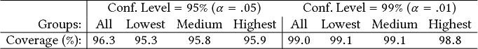 |
Overall, coverage probabilities are close to their confidence levels, although one can notice that the technique may produce conservative confidence intervals.
Second, we evaluate the technique on Fleiss’ $\kappa _F$ for individual referents (see Section 3.4), where we test all 42 referents of the study. We also evaluate it with random groups of referents. We test a total of 200 random groups, where half contain 5 referents, and the other half contain 10 referents. After $1,600$ iterations, results are as follows:
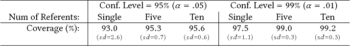 |
Each estimate is based on many samples, so we also report standard deviations. We observe that confidence intervals for individual referents are less precise, resulting in lower coverage probabilities with a larger variance. This is possibly due to larger deviations from the normality assumption as the number of referents becomes too low.
Finally, we evaluate the jackknife technique for differences in Fleiss’ $\kappa _F$ within the same group of participants. We test differences between individual references and between equal groups of four or eight referents. We run a total of $3 \times 50 = 150$ tests, and for each test, we compute the coverage probability of the jackknife confidence intervals for $1,600$ iterations:
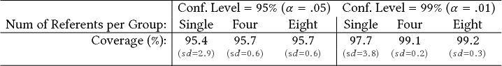 |
We observe again that confidence intervals may be less precise when comparing differences between individual referents.
Experiment 6.8. Evaluating the bootstrap method on populations generated by sampling with replacement is less appropriate because bootstrap confidence intervals are produced with the exact same approach. Furthermore, the method relies on a large number of resampling iterations so running large-scale Monte Carlo simulations on $\kappa$ coefficients requires significant computation resources. Therefore, we run a smaller experiment on the original dataset of Bailly et al. (2013).
Our method is as follows. We randomly divide the 20 participants of the study into two equal groups and count the number of referents for which the bootstrap confidence interval of their difference $\Delta \kappa _F$ does not include zero. We repeat this process a large number of times and calculate the mean error. This allows us to produce an estimate of the technique's Type I error rate. Due to computational constraints, we focus on a significance level of $\alpha = .05$ and limit the number of bootstrap iterations to $1,000$. We also set the number of times that we randomly partition participants into groups to 100. The mean number of referents for which the technique rejects the null hypothesis is 1.8, which corresponds to a Type I error rate of $1.8 / 42 = .043$.
6.6 Summary
The significance tests of the $V_{rd}$ and $V_b$ statistics yield large Type I errors. The jackknife technique is a good alternative for estimating within-participants agreement differences, while differences between independent groups of participants can be estimated with bootstrapping methods. The jackknife can be further used to construct confidence intervals for the overall $\kappa$ of a study and for the $\kappa$ of smaller groups of referents.
To the best of our knowledge, these techniques are the only viable solutions. However, they also have limitations. Depending on the source population, they may produce conservative confidence intervals or inflate Type I error rates when applied to agreement scores of individual referents. HCI researchers should be attentive to such limitations, in particular when they use small sample sizes and rely on statistical significance to draw conclusions.
7 REANALYSIS OF PAST GESTURE ELICITATION STUDIES
We reanalyze the results of four gesture elicitation studies, all published in the proceedings of CHI. Through our analyses, we demonstrate the use of chance-corrected coefficients and specific agreement. For estimation and hypothesis testing, we apply the resampling methods discussed in Section 6. We discuss how our analyses affect the authors’ original interpretation of their findings.
7.1 Bend Gestures for Flexible Displays – Lahey et al. (2011)
The gesture elicitation study by Lahey et al. (2011) explored a vocabulary of bend gestures for flexible portable displays. The investigators identified symmetrical pairs of actions (e.g., “open-close” and “play-pause”) and then looked for appropriate matchings with bend gesture pairs. Thus, signs represented gesture pairs rather than individual gestures.
The study involved 10 participants and was divided into three sessions. In Session 1, participants were asked to define eight unique bend gesture pairs. In Session 2, participants were presented seven action pairs, and for each, they had to propose a preferred bend gesture pair. Finally, in Section 3, they proposed a preferred gesture pair for a total of 10 action pairs of 5 mobile applications.
The investigators calculated agreement scores for both Sessions 2 and 3. Their average scores were $A=.326$ and $A=.368$, respectively, which correspond to $AR=.251$ (Session 2) and $AR=.298$ (Session 3). According to Vatavu and Wobbrock (2015), these values can be interpreted as medium agreement. However, Lahey et al. (2011) reached a different conclusion and argued that “the consensus on the mapping of those bend gestures to actions was overall low, showing that each participant had his or her own preference.” Given this assessment, the investigators did not propose any consensus gesture set. Is the investigators’ conclusion justified?
Table 10 presents chance-corrected agreement indices for Sessions 2 and 3. Both Fleiss’ $\kappa _F$ and Krippendorff's $\alpha$ are low, and their $95\%$ CIs range from negative to positive values. These results are in line with the investigators’ assessment: there is no evidence that participants have reached agreement. How can one explain this large discrepancy between agreement rates and chance-corrected indices? How did the investigators reach the right conclusion despite the fact that their $A$ scores were similar or higher than representative averages of older gesture-elicitation studies (Wobbrock et al. 2005, 2009)?
| A | AR | Fleiss’ $\kappa _F$ | Krippendorff's $\alpha$ | |
| Session 2 | .326 $[.186, .466]$ | .251 $[.093, .408]$ | .040 $[-.064, .144]$ | .054 $[-.049, .156]$ |
| Session 3 | .368 $[.269, .467]$ | .298 $[.186, .409]$ | .043 $[-.056, .141]$ | .052 $[-.045, .149]$ |
| Note: Brackets indicate $95\%$ jackknife CIs. Lahey et al. (2011) (in Table 4) report an $A_i=.66$ for the referent Contacts: Open-Close (Session 3). The correct value is .54, which results in a slightly lower average for $A$. |
||||
We conduct a more detailed analysis to answer these questions. Results show that participants reused a surprisingly small number of signs, i.e., gesture pairs. Three signs (“AB,” “CD,” and “CE”) accounted for $73\%$ of proposals in Session 2 and for $86\%$ of proposals in Session 3. We further analyze the number of agreement pairs for individual signs and find that these three signs alone explain $96\%$ of observed agreements for Session 2 and $99\%$ of observed agreements for Session 3. Although additional signs emerged during the study (a total of 15 additional signs for both sessions), those were used sporadically and with no coherence among participants. Furthermore, preferences over the three most frequent signs were still very divided for most referents, showing a highly arbitrary assignment of signs to referents. Our analysis of specific agreement confirms these trends. Figure 8 shows that specific agreement is either zero or extremely low for all but three very frequent signs (“AB,” “CD,” and “CE”). As $A$ and $AR$ do not account for such bias, they result in misleading agreement scores. Here, the investigators relied on intuition and common sense to reach the right conclusion.
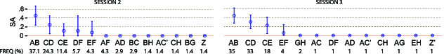
Despite these results, the authors still characterize bias as agreement: “participants express strong agreement when designing individual bend gestures as well as bend gesture pairs” (Lahey et al. 2011). To reach this conclusion, they observe the frequency distribution of gestures produced in Session 1, where this distribution demonstrates a clear overall preference for a few gesture pairs. As we discussed in Section 3.5, inspecting the frequency distribution of observed signs is possibly the best approach for identifying overall preferences. Agreement rates and $\kappa$ coefficients are not suitable for this type of analysis.
Polarity of bend gestures. Lahey et al. (2011) further explored how participants agreed on the polarity of proposed bend gestures, where polarity is “either up (toward the user) or down (away from the user).” They reported that “for actions with a strong directional cue, we found strong consensus on the polarity of the bend gestures.” They also claimed that for Session 3, “the majority of the bend gesture pair/action pair mappings were consistent in terms of their polarity.”
However, these conclusions were not justified by using formal statistics. Agreement indices can help us assess to what extent statistics support them. We reanalyzed the data by first removing proposals for which polarity did not conform to the above definition. We removed $8.6\%$ of proposals for Session 2 and $6.0\%$ of proposals for Session 3. Table 11 presents our results for the full set of referents and, separately, for directional referents only: Next/Previous, Left/Right, Up/Down, and Zoom In/Out. Fleiss’ $\kappa _F$ and Krippendorff's $\alpha$ are not useful in this case, as the two polarity categories always appear in pairs with the same frequency. Instead, we use Brennan–Prediger's $\kappa _q$ with $q = 2$, which calculates chance agreement as $p_e = .5$. This high ($50\%$) probability that pairs of participants agreed by chance explains the large discrepancy between $AR$ scores and Brennan–Prediger's $\kappa _q$.
| Referents | A | AR | Brennan–Prediger's $\kappa _q$ | |
| Session 2 | All | .662 $[.540, .783]$ | .619 $[.475, .763]$ | .238 $[-.050, .527]$ |
| Directional | .752 $[.568, .936]$ | .720 $[.499, .940]$ | .439 $[-.002, .881]$ | |
| Session 3 | All | .622 $[.533, .711]$ | .576 $[.474, .677]$ | .151 $[-.052, .355]$ |
| Directional | .669 $[.557, .780]$ | .626 $[.497, .756]$ | .252 $[-.007, .511]$ | |
| Note: Brackets indicate $95\%$ jackknife CIs. |
||||
Overall, the results do not support the investigators’ conclusions or at least, they are nonconclusive. The low statistical power of the study (10 only participants) results in wide confidence intervals for Brennan–Prediger's $\kappa _q$, which means that estimations are highly uncertain. Table 12 presents differences in agreement scores between directional and nondirectional referents. Again, these results do not show any clear difference between the two referent groups.
| A | AR | Brennan–Prediger's $\kappa _q$ | |
| Session 2 | .157 $[-.035, .350]$ | .176 $[-.053, .404]$ | .351 $[-.105, .808]$ |
| Session 3 | .051 $[-.074, .176]$ | .053 $[-.092, .197]$ | .105 $[-.183, .394]$ |
| Note: Brackets indicate $95\%$ jackknife CIs. |
|||
7.2 Single-Hand Microgestures – Chan et al. (2016)
Chan et al. (2016) conducted a gesture elicitation study to explore the design of SHMGs. This study is one of the first to report $AR$ (instead of $A$) and to closely follow the interpretation of agreement rates proposed by Vatavu and Wobbrock (2015). Specifically, Chan et al. (2016) reported an average $AR=.191$ and interpreted this value as medium agreement. This allowed them to define a consensus gesture set, consisting of eight unique signs for a total of 35 referents. They then extended this set to 16 unique signs based on variations of those signs.
The interpretation given by Chan et al. (2016) does not consider the problem of chance agreement. During their analysis, the investigators observed that participants frequently mixed up the number of fingers used. To deal with this issue, they separated “gestures that used two or less fingers from those with three or more fingers.” By relaxing the constraints on how signs were classified as similar or different, the investigators succeeded in increasing agreement rates, as agreement now reflected a smaller number of gesture parameters. However, as this strategy constrains the vocabulary of active signs, it may as well increase chance agreement.
We reanalyzed the 560 gesture proposals (16 participants $\times$ 35 referents) as identified by Chan et al. (2016).7 Table 13 presents estimates of overall agreement scores. Chance-corrected coefficients are particularly low, while Fleiss’ $\kappa _F$ $95\%$ CI includes zero. These agreement values are slightly higher than ones calculated for the previous study of Lahey et al. (2011), and proponents of significance tests could argue that chance-corrected agreement is (at least marginally) significantly higher than zero. However, statistical significance by itself provides very little information about the level of observed agreement. A closer look into the results of the study shows that participants tended to prefer tap-like microgestures for referents that represent discrete actions such as “select single,” and swipe-like microgestures for referents that represent continuous actions such as “scrolling.” Yet, apart from those two referents, results do not clearly show that participants reached consensus (see Figure 9). For example, for referents that represented discrete but directional actions, e.g., “previous” and “next,” preferences were highly divided between swipe and tap-like microgestures.
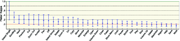
| A | AR | Fleiss’ $\kappa _F$ | Krippendorff's $\alpha$ |
| .242 $[.137, .347]$ | .191 $[.079, .304]$ | .091 $[.000, .182]$ | .093 $[.002, .183]$ |
| Note: Brackets indicate $95\%$ jackknife CIs. |
|||
Our analysis further indicates that there was a bias toward a small number of signs. Among the 46 unique signs defined by the investigators, a single sign (tap thumb with two or less fingers) represented alone $23\%$ of all proposals and accounted for $38\%$ of all observed agreements. Moreover, the four most frequent signs represented $59\%$ of all proposals and accounted for $82\%$ of all agreements. Figure 10 further shows that specific agreement is spread over a small number of signs. For less frequent signs, agreement is generally low, with two notable exceptions: the 12${\text{th}}$ sign (tap two or less fingers) and the 15${\text{th}}$ sign (tap thumb and more than two fingers). Agreement over these two signs is relatively high despite their low frequency. In such cases, agreement is less likely to have occurred by chance.
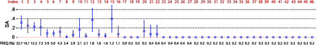
Bias toward a small number of signs can also produce conflicts. In particular, the most popular proposal for 30 out of 35 referents was within four only signs. To resolve such conflicts, the investigators re-examined their data to identify recurring patterns in participants’ use of individual fingers. Based on such patterns, they produced new gesture variations. This approach allowed the investigators to combine observations from real data and their own design skills to give a solution to a rather complex design problem. Yet, agreement scores only partially reflect the final consensus gesture set where such variations are present. We discuss methodological issues related to the analysis of sign vocabularies in Section 8.
7.3 On-Skin Gestures – Weigel et al. (2014)
Weigel et al. (2014) conducted a gesture elicitation study to explore a vocabulary of on-skin gestures. The study investigated a large, open-ended design space that involved diverse input modalities (multitouch, grab, pull, press, scratch, shear, squeeze, twist) and several locations on the upper limb (fingers, wrist, back of the hand, palm, forearm, elbow, upper arm). A total of 22 volunteers participated in the study and proposed gestures for a total of 40 referents, where 33 referents represented common commands and seven referents represented expressions of emotions. The investigators calculated individual per-referent $A_i$ agreement scores, which ranged from .08 to .69. The overall average was $A=.25$, which corresponds to $AR = .21$. As those values were close to the ones of other related gesture elicitation studies (Lee et al. 2010; Wobbrock et al. 2009), Weigel et al. (2014) argued: “scores are comparable with those in prior work […], despite the larger input space of our study.”
However, a larger input space does not always lead to lower chance agreement because participants may disregard the extra input modalities and only agree on a small set of obvious gestures. For example, the five highest agreement scores that Weigel et al. (2014) report for command gestures correspond to common direct-manipulation gestures dedicated to content rotation and resizing actions. As these gestures are widely available on today's multitouch devices, the authors acknowledge: “these findings show that participants transferred conventional multitouch gestures to on-skin input.” For the rest of the commands, agreement scores ($A_i$) were considerably lower, with a highest value of .31, where again, agreement was largely due to the use of conventional multitouch gestures. Furthermore, agreement depends on the strategy that investigators follow to classify gesture descriptions to signs. The higher the granularity of the classification process, the harder it is to reach agreement, since participants need to agree on a larger number of gesture parameters. Our following analysis attempts to account for these issues.
Weigel et al. (2014) identify three dimensions that describe an on-skin gesture: (i) the body location on which the gesture takes place, e.g., fingers, palm, and forearm, (ii) its input modality, e.g., multitouch, grab, and twist, and (iii) other gesture properties, e.g., number of fingers, direction, and movement dynamics.
On-body location. We first investigate if participants agreed on the on-body location of gestures by considering eight basic locations (upper arm, elbow, forearm, back of the hand, palm, fingers, wrist, and shoulder), as well as combinations of multiple locations (e.g., palm + fingers). After inspecting Fleiss’ $\kappa _F$ and Krippendorff's $\alpha$ in Table 14, we conclude that participants did not reach consensus. Again, the $A$ and $AR$ indices provide very misleading information about the level of intrinsic agreement.
| A | AR | Fleiss’ $\kappa _F$ | Krippendorff's $\alpha$ | |
| On-body location | .328 $[.252, .404]$ | .296 $[.216, .376]$ | .004 $[-.016, .024]$ | .005 $[-.015, .025]$ |
| Input modality | .336 $[.297, .375]$ | .304 $[.263, .345]$ | .119 $[.085, .154]$ | .120 $[.086, .155]$ |
| Note: Brackets indicate $95\%$ jackknife CIs. $A$ scores are not consistent with the ones reported by Weigel et al. (2014) because we follow a different approach to classify proposals into signs. |
||||
Input modality + other gesture properties. The original agreement analysis of Weigel et al. (2014) disregarded the on-body gesture location and focused on the input modality of the gesture in combination with individual gesture properties. For example, all the “pinch” gestures were classified as identical, regardless of whether they were executed on the palm or the forearm. To assess if different gesture proposals belonged to the same unique sign, the investigators considered various movement properties, such as the gesture direction or its force and intensity, e.g., tapping with force vs. tapping gently. However, other properties, such as the number of fingers, were generally not considered. Unfortunately, the classification strategy that the investigators followed is not fully known.
For our analysis, we relied on textual gesture descriptions, i.e., textual tags provided by the authors in a spreadsheet. These textual tags were used by the investigators to describe individual gesture proposals. They principally represent input modalities, but for some modalities, the touch modality in particular, they describe additional variations. Representative examples of such tags are: tap, slide, slide/swipe, poke, scratch, squeeze+shake, tap+twist, and so on. We extracted these tags directly from the spreadsheet and handled them as signs. Unfortunately, these signs do not coincide with the actual signs considered by the investigators to calculate agreement. As a result, our analysis does not reproduce the actual agreement scores reported by Weigel et al. (2014).
Overall, we counted 65 unique signs, but only 21 of those signs had at least one agreement. Table 14 (Input Modality) presents agreement scores calculated over the full set of referents. Interestingly, our average $A$ is considerably higher than the one ($A=.25$) reported by Weigel et al. (2014). The reason is that our gesture classification is less stringent, causing agreement to happen more easily. At the same time, this approach increases the probability of agreement by chance, which explains the large discrepancy between the overall agreement rate and chance-corrected coefficients. A more detailed analysis shows that the slide sign alone represented $43\%$ of all proposals and was responsible for $80\%$ of all observed agreements. Tap was the second most popular sign ($14\%$), while twist was the most popular ($4\%$) skin-specific sign. Figure 11 shows how the slide sign and its variations dominated participants’ proposals and agreement scores. There was little or no consensus for other signs, where poke-tap and punch are the only skin-specific signs for which there is evidence of agreement. Figure 12 presents Fleiss’ $\kappa _F$ for individual referents by preserving the authors’ original presentation order. Notice that $\kappa _F$ is particularly high for five referents that correspond to direct content-manipulation actions (“enlarge,” “shrink,” “rotate,” “zoom-in,” “zoom-out”).
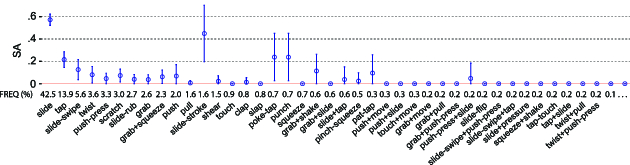
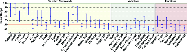
The gesture classification approach can greatly affect agreement scores. For example, for the “sympathy” referent, we decided to discriminate between the slide-rub and slide-stroke modalities, as they appear as different in the investigators’ spreadsheet. In contrast, Weigel et al. (2014) most likely grouped them under a common sign, and this resulted in a higher agreement score. If we follow their approach, the Fleiss’ $\kappa _F$ for this referent will be .41, $95\%$ CI $=[.06, .77]$. More generally, agreement scores have little value by themselves. In order to interpret them, one needs to know exactly what participants agree upon, i.e., know how signs are defined and how proposals are classified into these signs. We further discuss this issue in Section 8.
7.4 Keyboard Gestures – Bailly et al. (2013)
Bailly et al. (2013) investigated gestural shortcuts for their Métamorphe keyboard. Métamorphe is a keyboard with actuated keys that can sense user gestures, such as pull, twist, and push sideways. The study was later reanalyzed by Vatavu and Wobbrock (2015, 2016); thus, it provides a good basis for comparisons.
In this study, 20 participants suggested a keyboard shortcut for 42 referents on a Métamorphe mockup. Proposing a shortcut required choosing (i) a key and (ii) the gesture applied to the key. Bailly et al. (2013) treated shortcuts as a whole but also analyzed keys and gestures separately. Here, we analyze keys and gestures separately. Participants produced a total of 71 different signs for keys and 27 different signs for gestures.8
Table 15 shows overall agreement scores for keys and for gestures. An investigator who uses the $A$ or $AR$ measures may infer that participants’ consensus was higher for gestures than for keys. However, chance-corrected coefficients reveal that this difference is most likely due to chance agreement. As the number of signs was lower for gestures than for keys and participants exhibited a strong bias for the “top push” sign, agreement was more likely to occur by chance. Overall, the “top push” sign represented $28\%$ of proposals and was alone responsible for $37\%$ of observed agreements. Figure 13 presents the specific agreement for individual gestures. Although the “top push” sign dominated participants’ proposals, the distribution of specific agreement is more uniform across signs than in our previous case studies. Furthermore, the evidence that agreement is above zero is high for most signs of interest. These trends explain the higher chance-corrected agreement scores that we found for this study.
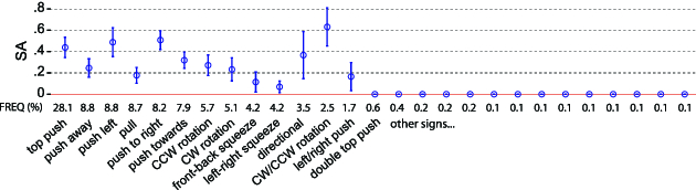
| A | AR | Fleiss’ $\kappa _F$ | Krippendorff's $\alpha$ | |
| Keys | .320 $[.213, .427]$ | .284 $[.172, .397]$ | .260 $[.148, .371]$ | .261 $[.149, .372]$ |
| Gestures | .370 $[.323, .417]$ | .336 $[.287, .386]$ | .240 $[.192, .289]$ | .241 $[.193, .289]$ |
| Note: Brackets indicate $95\%$ jackknife CIs. |
||||
We can also use confidence intervals to back up the authors’ claim on the effect of directional referents on agreement: “highly directional commands […] tended to have a high gesture agreement” (Bailly et al. 2013). The difference in Fleiss’ $\kappa _F$ between the eight directional referents containing the terms top, bottom, left, right, previous, or next and all other referents is $\Delta \kappa _F = .41$, $95\%$ CI $=[.24, .58]$, so the evidence supporting this claim is overwhelming.
Women vs. Men. Bailly et al. (2013) collected proposals from 11 women and 9 men. Vatavu and Wobbrock (2016) reanalyzed their dataset to test differences in agreement between genders but observed similar overall agreement rates between women and men (.353 vs. .322). If we use Fleiss’ $\kappa _F$ to estimate this difference, we find that $\Delta \kappa _F=.06$, $95\%$ CI $=[-.11, .16]$, where we use the bootstrap method to construct the confidence interval. Vatavu and Wobbrock (2016) continued their analysis and used the $V_b$ statistic to compare agreement differences between genders for individual referents. They found9 “significant differences ($p\lt.05$) for 7 referents.” Based on this finding, they concluded: “these results show that women and men reach consensus over gestures in different ways that depend on the nature of the referent […]”
We showed, however, that the Type I error rate of the $V_b$ test is unacceptably high (see Section 6); thus, such differences may be random, rather than the result of a gender effect. To verify the conclusion of Vatavu and Wobbrock (2016), we run a simulation experiment over the original dataset of Bailly et al. (2013). The experiment draws inspiration from permutation tests (Hesterberg et al. 2005). It evaluates the $V_b$ test on participant groups that are randomly chosen from the pool of the 20 participants of the original study. There are $(\scriptsize{\begin{array}{c}{20}\\{9}\end{array}})=167{,}960$ ways to partition 20 participants into two independent groups of 9 and 11 participants. Since testing all these partitions can be extremely long, we randomly create $1{,}000$ such partitions. We then apply the $V_b$ test to each random partition and count the number of referents for which the difference between the $AR$ of the two groups is significantly different than zero ($\alpha = .05$).
The results confirm our concerns. The mean number of referents per partition for which the null hypothesis is rejected is 8.8 ($sd = 2.6$). Therefore, the seven referents that Vatavu and Wobbrock (2016) report when comparing agreement between women and men is a well-expected result, below the average number of significant differences observed for fully random partitions. The Type I error rate of the $V_b$ test for this dataset can be estimated as $8.8 / 42 = .21$, which is again very high, more than four times higher than its nominal value.
For comparison purposes, we re-evaluate the bootstrap method with the exact same procedure.10 We produce $95\%$ confidence intervals by using $3{,}000$ bootstrap samples, and for each confidence interval, we reject the null hypothesis if the interval does not include zero ($\alpha = .05$). The mean number of referents per partition for which the method rejects the null hypothesis is 1.94, which gives a Type I error rate of $1.94 / 42 = .046$. This error rate is very close to the one we found in Experiment 6.8 and further confirms the good behavior of the bootstrap method.
Can we then use the method to test gender differences for individual referents? We discourage such practices for several reasons. Making comparisons between women and men was out of the scope of the original study of Bailly et al. (2013). The size of the two groups was particularly low, while the study did not control for confounding variables, such as computer skills or experience with novel input devices, which might highly correlate with gender. We argue against making unplanned post-hoc comparisons over uncontrolled samples of such small sizes, as those can result in misleading conclusions. Furthermore, jackknife and bootstrap confidence intervals for individual referents may not be precise, especially when sample sizes are low. As a result, using them to test such hypotheses may not be appropriate.
7.5 Synthesis of Findings
Results from the four case studies confirm that the $AR$ index is problematic. In several cases, it provides misleading information about the level of consensus reached by participants. Table 16 combines the results of Tables 10, 13, 14, and 15. We observe that similar $AR$ scores can result in very different chance-corrected values.
| Case study | A | AR | Fleiss’ $\kappa$ | Krippendorff's $\alpha$ |
| Lahey et al. (2011) | .326 $[.186, .466]$ | .251 $[.093, .408]$ | .040 $[-.064, .144]$ | .054 $[-.049, .156]$ |
| .368 $[.269, .467]$ | .298 $[.186, .409]$ | .043 $[-.056, .141]$ | .052 $[-.045, .149]$ | |
| Chan et al. (2016) | .242 $[.137, .347]$ | .191 $[.079, .304]$ | .091 $[.000, .182]$ | .093 $[.002, .183]$ |
| Weigel et al. (2014) | .328 $[.252, .404]$ | .296 $[.216, .376]$ | .004 $[-.016, .024]$ | .005 $[-.015, .025]$ |
| .336 $[.297, .375]$ | .304 $[.263, .345]$ | .119 $[.085, .154]$ | .120 $[.086, .155]$ | |
| Bailly et al. (2013) | .320 $[.213, .427]$ | .284 $[.172, .397]$ | .260 $[.148, .371]$ | .261 $[.149, .372]$ |
| .370 $[.323, .417]$ | .336 $[.287, .386]$ | .240 $[.192, .289]$ | .241 $[.193, .289]$ | |
| Note: Brackets indicate $95\%$ jackknife CIs. |
||||
The source of such discrepancies is the difference in size of different sign vocabularies or, more generally, bias in the frequency distribution of signs. Figure 14 presents the observed bias distribution for each study. For each bias distribution, the figure also presents our closest model of bias based on a Zipf–Mandelbrot or a half-normal probability distribution (see Section 3.2). We experimentally determined the bias parameters ($B$ or $sd$) of these functions such that the chance agreement they produce approximates Fleiss’ $p_e$. Notice that chance agreement can be particularly high. For example, chance agreement is over $20\%$ for the studies of Lahey et al. (2011) and Weigel et al. (2014). In contrast, bias for keys was very low in the study of Bailly et al. (2013). Chance agreement was very low ($p_e = .03$) in this case, despite the fact that the number of keys in a physical keyboard is hard-constrained.
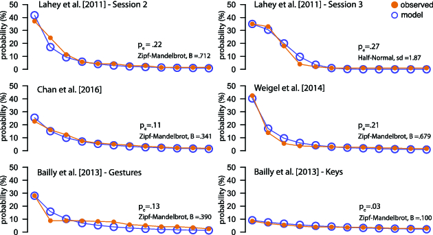
We already discussed that bias may reveal overall preferences over highly usable gestures and help investigators disregard gestures that participants seem to avoid. For example, Lahey et al. (2011) did not find clear mappings between referents and signs, but the study helped them identify strong preferences for a small set of bend-gesture pairs. In other cases, bias may not be a desired artifact. In the study of Weigel et al. (2014), participants’ proposals were highly dominated by signs that correspond to common multitouch gestures, thus bias was partly due to legacy bias (Morris et al. 2014). Finally, in the study of Bailly et al. (2013), bias was largely due to the frequent use of the obvious “top push” as a default sign, which might have happened when participants could not think of meaningful associations between commands and key gestures.
Regardless of the source of bias, chance-corrected agreement indices allow researchers to isolate its effect on agreement and analyze it independently from agreement that considers the semantics of referents. When participants cannot differentiate among referents, so clear mappings between signs and referents do not emerge, chance-corrected agreement is expected to be low. In such cases, it may be wiser to investigate gesture customization approaches (Oh and Findlater 2013), instead of insisting on unique mappings that cannot be characterized as “user-defined.”
In addition to bias, we analyze how sign preferences are distributed in the proposals of individual referents in all four studies. To this end, we collect proposals for a total of 156 referents. For the study of Bailly et al. (2013), we count proposals for both gestures and keys. For the study of Lahey et al. (2011), we count proposals for both Sessions 2 and 3. We then group referents into four ranges of agreement according to their observed agreement rate $AR_i$, where $AR_i \in [.1, .3]$, $[.3, .5]$, $[.5, .7]$ or $[.7, .9]$. For each referent, we rank the proposed signs based on their relative frequencies and then aggregate these frequencies over all the referents of each agreement range to produce an overall probability distribution of sign preferences (see Section 6.1).
Figure 15 summarizes our results, where for each observed distribution, we also show the Zipf–Mandelbrot model that approximates the mean $AR_i$ of the group. The bottom part of the figure shows the same distributions with log–log plots. Such plots are commonly used to illustrate how well observed frequencies follow a power-law model (Newman 2005). Although we only vary a single model parameter, the observed sign frequencies are generally close to our Zipf–Mandelbrot models. This is clearer for the highest frequency ranks that dominate agreement. We acknowledge that the probability estimation for lower ranks is more noisy and uncertain, but the contribution of rare signs to agreement is negligible. More precise power-law models require the analysis of larger participant samples. This is out of the scope of this article, but it is an interesting future direction.
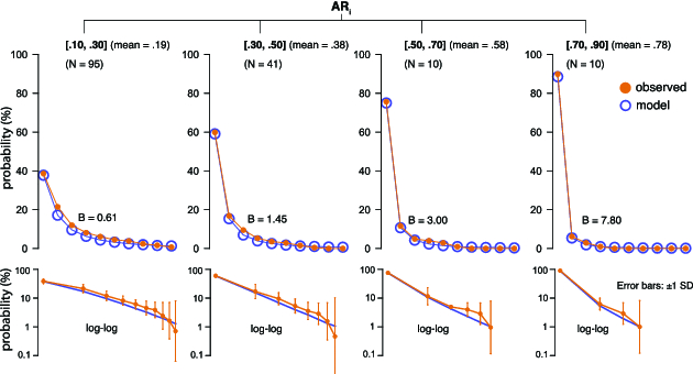
8 METHODOLOGICAL ISSUES
Agreement largely depends on the process investigators follow to classify participant proposals. This process requires first defining a sign vocabulary and then using this vocabulary to classify observed gestures. We discuss methodological issues that HCI researchers should consider when they carry out these tasks.
8.1 Defining a Sign Vocabulary
An agreement value cannot be interpreted unless a clear frame of reference is provided because one needs to know what participants agree upon. Therefore, sign vocabularies need to be well defined, e.g., through an identity or a similarity measure that clearly determines if any two gesture descriptions belong to the same or two distinct signs.
Defining a sign vocabulary is rarely a straightforward process. For their key gestures, Bailly et al. (2013) started with a closed set of 10 distinct gesture signs, but several participants invented additional signs during the study, where most were combinations or variations of the original set. The investigators included them in their analysis, but as many of them appeared rarely, they classified them under larger groups (“combo” and “other”). Chan et al. (2016) faced a more challenging problem as they studied an open-ended vocabulary, where gesture variations was the result of a complex combination of different parameters, such as the number and type of active fingers, their poses, their relative movements, and compound gestures. To deal with this complexity, the investigators simplified their gesture classification criteria by reducing the number of gesture parameters. This approach helped the authors focus on gesture properties for which consistent behavior, i.e., some reasonable level of consensus, among participants was observed. Weigel et al. (2014) followed a similar approach. However, we could not reproduce the agreement values that the authors reported because the similarity criteria that they used to classify gestures were ill-defined. Since their agreement values do not have a clear frame of reference, they are hard to interpret.
In the above examples, the investigators construct the sign vocabulary a-posteriori, often by inspecting the entire dataset. This approach raises some questions. Is the vocabulary definition general enough to apply to a different collection of gesture descriptions? Does it inform design or is it simply conceived to maximize agreement? An in-depth discussion of these questions is out of the scope of this article, but there are strategies that could partially address them. For example, a good practice is to specify the sign vocabulary prior to the data analysis based on existing theory, previous evidence, or pilot studies. Creating a gesture taxonomy (Wobbrock et al. 2009) to explore the design space of possible gestures and identify their dimensions and categories could help to this direction. Another strategy is to assign the task to multiple investigators or ask external experts to verify the sign definition approach.
Finally, we recommend that investigators inspect gesture descriptions in a random order by hiding their referents. Given this approach, any bias in the sign-definition and classification process will appear as overall referent-independent bias, and chance-corrected indices will eliminate its effect on agreement. The approach may also discourage data-analysis strategies that artificially optimize agreement.
8.2 Classifying Participants’ Proposals Into Signs
Gesture classification is typically performed by humans. Since this process can rely on subjective criteria, its reliability needs to be verified. In the previous sections, we investigated agreement indices for assessing consensus among participants. However, the exact same indices can be used to verify the reliability of gesture classification results. We explain the approach with our fictitious study on user-elicited grasps (see Section 2). Imagine that three independent coders review the video recordings of a random sample of 10 grasp proposals (G1–G10) and classify them into unique signs. Suppose Table 17 summarizes their results.
| G1 | G2 | G3 | G4 | G5 | G6 | G7 | G8 | G9 | G10 | Total | |
| A | 0 | 0 | 0 | 0 | 0 | 0 | 0 | 0 | 0 | 0 | 0 |
| B | 3 | 0 | 3 | 0 | 0 | 0 | 0 | 3 | 0 | 2 | 11 |
| C | 0 | 3 | 0 | 0 | 3 | 0 | 3 | 0 | 0 | 1 | 10 |
| D | 0 | 0 | 0 | 2 | 0 | 1 | 0 | 0 | 2 | 0 | 5 |
| E | 0 | 0 | 0 | 1 | 0 | 2 | 0 | 0 | 1 | 0 | 4 |
| Note: Three independent coders classify a sample of 10 random grasp descriptions (G1–G10) through video analysis. Each cell gives the number of coders who classify a grasp into a specific sign. For those 10 grasp descriptions, the three coders have made use of four unique signs (“B,” “C,” “D,” “E”). |
|||||||||||
To verify the reliability of this classification, we assess how the three coders agree with each other. To this end, we calculate Fleiss’ $\kappa _F$: the percent agreement is $p_a=.733$, the chance agreement is $p_e=.291$, and therefore $\kappa _F = .624$. This $\kappa _F$ value is a measure of reliability. A low score may require the investigators to update their sign definitions and rerun the classification process. For example, the investigators may decide to group the signs “D” and “E” together because distinguishing between them seems to be difficult or highly random.
Notice that $\kappa _F$ is calculated over the exact same sign vocabulary that we used to calculate agreement among the participants of the study (see Table 1). As before, one may assume an infinite vocabulary of signs ($q\rightarrow \infty$) from which coders choose, and bias has the exact same effect on chance agreement. Here, the role of chance-corrected coefficients is to ensure that coders differentiate among cases – they do not simply assign the most prevalent signs in random. Although we use the same indices, the assumptions for constructing their confidence intrervals are now different. Coders are shown gesture descriptions (not referents), and those should not be considered as fixed. For a detailed explanation of how to construct confidence intervals in this case, we refer the reader to Gwet's (2014) handbook.
Gesture elicitation studies that have used $\kappa$ coefficients to verify the reliability of their gesture classification results, either fully or for part of their analysis, include the studies of Micire et al. (2009), Gleeson et al. (2013), Weigel et al. (2014), and Troiano et al. (2014). Classifying proposals to signs can be especially tedious and time-consuming, but previous work (Grijincu et al. 2014) has developed crowdsourcing methods to facilitate this task.
9 LIMITATIONS AND FUTURE WORK
There are issues that this article has not addressed. We discuss limitations of our analysis and identify directions for future work.
9.1 Complex Gesture Elicitation Designs
Gesture elicitation can employ complex design features that are not well supported by the statistics that we discussed in this article. For example, previous work (Morris 2012) has examined experimental protocols that allow participants to propose multiple gestures per referent. Such designs are not unique to gesture elicitation. For example, Gwet (2014) discusses similar scenarios in the field of medical coding, where coders assign multiple codes to each item, sometimes by order of priority. In these scenarios, intercoder agreement can be assessed by reorganizing the data and using weighted $\kappa$ coefficients (Gwet 2014), where weights express varying degrees of agreement or disagreement. Gwet (2014) also discusses indices that measure agreement with respect to a gold standard. In the context of gesture elicitation, such indices could be used to assess how participants’ proposals agree with a state-of-the-art vocabulary or, alternatively, with a vocabulary specified by a design expert.
Other study designs may violate certain assumptions of standard agreement indices. In particular, the use of nonoverlapping gestures sets and semantic grouping (Bailly et al. 2013; Piumsomboon et al. 2013) may affect the way chance agreement is estimated, as the gestures proposed by participants for different referents may not be assumed as independent. Future work needs to study alternative probabilistic models that account for inter-referent relationships and constraints.
9.2 Symbolic Gestures vs. Direct-Manipulation Actions
The four gesture elicitation studies that we reanalyzed focus on vocabularies of symbolic or abstract gestures, which usually serve as shortcuts to discrete, noncontextual operations. However, several studies (Wobbrock et al. 2009; Piumsomboon et al. 2013) have investigated contextual, direct-manipulation gestures. In such studies, the problem of chance agreement may be lower because direct-manipulation operations such as selection, manipulation, and transformation, have unique constraints (e.g., continuous vs. discrete control and spatial constraints), which may make bias and conflicts across different referents less likely to happen.
This hypothesis remains to be verified. Although Piumsomboon et al. (2013) provided access to their gesture classification spreadsheet, we could not use it to assess chance-corrected (or specific) agreement. The reason is that their classification approach compares gestures on a per-referent basis but does not result in a common sign vocabulary for all referents. Since gestures are not comparable for similarity across referents, we cannot produce a contingency table as in Table 2 to compute chance-corrected (Equation (5)) or specific agreement (Equation (6)).
9.3 Characterizing Low or High Agreement
The article does not provide any guidelines about which levels of chance-corrected agreement can be considered as high or low. We acknowledge, however, that interaction designers and HCI researchers may need to use such guidelines in order to take concrete design decisions. For example, which levels of $\kappa$ justify the definition of user-defined mappings between referents and signs? When should designers opt for a customization-based approach? These questions require further research effort and a more systematic evaluation of the costs and benefits of user-defined gestures (e.g., see the study by Morris et al. (2010)) under various agreement levels. We thus leave this direction as future work.
10 CONCLUSIONS
We reviewed statistical methods for agreement assessment in gesture elicitation studies. We investigated three major questions: (i) how to measure agreement; (ii) how to interpret agreement values; and (iii) how to support statistical inference. Our conclusions can be summarized as follows:
- The agreement rate $AR$ (Vatavu and Wobbrock 2015) and its approximation $A$ (Wobbrock et al. 2005) do not account for chance agreement and can lead to overoptimistic conclusions about the true level of consensus reached by participants. We recommend the use of $AR$ in combination with Fleiss’ $\kappa _F$ or Krippendorff's $\alpha$. These indices can be complemented with indices of agreement specific to signs (Spitzer and Fleiss 1974; Uebersax 1982). A careful analysis of the observed bias distribution is also highly recommended.
- The recommendations of Vatavu and Wobbrock (2015) for assessing the magnitude of agreement rates can lead authors to incorrectly interpret their agreement scores. Unfortunately, objective measures for assessing what levels of agreement are high, or sufficient to justify the selection of user-defined gesture vocabularies do not currently exist. This is a challenging future direction.
- The $V_{rd}$ and $V_b$ significance tests (Vatavu and Wobbrock 2015, 2016) rely on problematic probabilistic assumptions and yield extremely high Type I error rates. We recommend instead the use of confidence intervals for estimation and hypothesis testing. Confidence intervals can be constructed with well-known jackknifing and bootstrapping methods.
In addition to the above questions, we discussed methodological issues concerning the gesture classification process. Gesture elicitation studies are extremely useful but can be complex to set up and analyze. The proper methodology that can ensure reliability and scientific rigor largely remains to be developed. To this end, the HCI community can gain a lot by considering lessons learned in other disciplines where similar issues have been addressed, instead of attempting to develop its own solutions in isolation.
ACKNOWLEDGMENTS
Completing this work would not be possible without the help of Pierre Dragicevic, who has dedicated significant time and effort into long discussions and has contributed both R code and textual content. The present article is partly based on our technical report (Tsandilas and Dragicevic 2016). I would also like to thank Gilles Bailly, Edwin Chan, Audrey Girouard, Thammathip Piumsomboon, Martin Weigel, and their supervisors or co-authors for sharing their data with us and allowing us to reanalyze their results. I am also grateful to Gilles Bailly for his feedback on an earlier version of this article, to Anastasia Bezerianos for many insightful comments, and to Wendy Mackay and Michel Beaudouin-Lafon for their advice.