The MARKOV package : Markovian models

Markovian models are the simplest, easiest to use statistical models available for genomic sequences. Statistical properties associated with a Markovian model make it become a valuable tool to the one who wants to take into account the occurrences of $k$-mers in a sequence. Their most commonly used version, the so-called classical Markovian models, can be automatically built from a set of real genomic sequences. Hidden Markovian models are now supported by GenRGenS at the cost of some preprocessing, as shown in section 3.1.3. Apart from genomics, such models appear in various scientific fields including-but-not-limited-to speech recognition, population processes, queuing theory and search engines^3.1.

Some theoretical aspects

Main definition

Formally, a classical Markovian model applied to a set of random variables $V_1,\ldots,V_n$ causes the probabilities associated with the potential values for $V_n$ to depend on the values of $V_{i},\ldots,V_{n-1}$. We will focus on homogenous Markovian models, where the probabilities for the different values for $V_n$ are conditioned by the values already chosen for a small subset $[V_{i-k-1},V_{i-1}]$ of variables from the past, also called context of $V_i$. The parameter $k$ is called the order of the Markovian model. Moreover, the probabilities of the values for $V_i$ in an homogenous Markovian model cannot in any way be conditioned by the index $i$ of the variable.

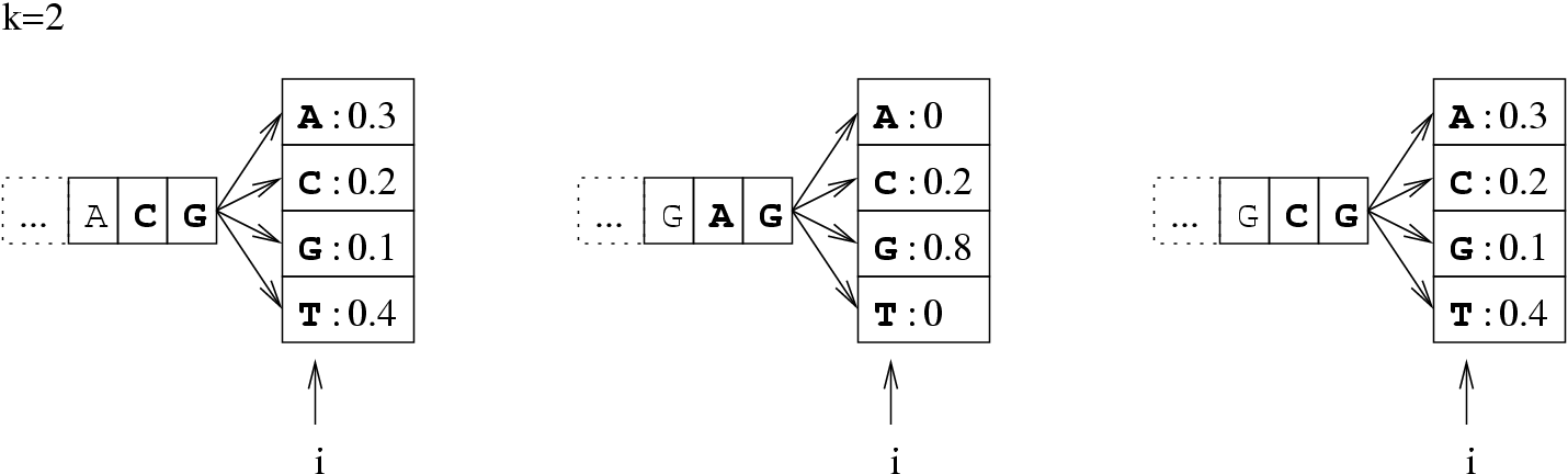
Figure 3.1: The probability of the event : "the $i$-th base is an $a$" depends on its $k$ predecessors.

Applied to genomic sequences, the random variable $V_i$ stands for the $i^{th}$ base in the sequence. The Markovian model constrains the occurrence probability for a base $\alpha$ in a given context composed of the $k$ previously assigned letters, therefore weakly^3.2! constraining the proportions of each $k+1$-mers.

What about heterogeneity ?

GenRGenS handles a small subset of the heterogenous Markovian class of models.
Formally, an heterogenous model allows the probabilities associated with a variable $V_i$ to depend on any of the variables prior to $V_i$. Our subset of the heterogenous Markovian models will use an integer parameter called $phases$ to compute the probabilities for $V_i$. The phase of a variable $V_i$ is simply given by the formula $i \mod phases$. In our subset of the heterogenous Markovian models, the probabilities for $V_i$ depend on both context and phase of the variable. Such an addition is useful to model phenomenons in which variables are gathered in packs of $phases$ consecutive variables, and their values not only depend of their contexts, but also of their relative position inside the pack. Such are sequences of protein-coding DNA, where the position of a base inside of a base triplet is well-known to be of interest.

It is also possible to simulate such phase alternation by introducing dummy letters encoding the phase in which they will be produced. For instance, an order 0 model having 3 phases (for coding DNA...) would result in a sequence model over the alphabet {$a_0$,$c_0$,$g_0$,$t_0$,$a_1$,$c_1$,$g_1$,$t_1$,$a_2$,$c_2$,$g_2$,$t_2$} having non-null transition probabilities only for $\cdots x_0\to y_1$, $\cdots x_1\to y_2$ and $\cdots x_2\to y_0$. Therefore, the expressivity of our heterogenous models do not exceed that of the homogenous ones, but it is much more convenient to write these models using an heterogenous syntax.

Hidden Markovian Models (HMMs)

Hidden Markovian models address the hierarchical decomposability of most sequences.

An hidden Markovian model is a combination of a top-level Markovian model and a set of bottom-level Markovian models, called hidden states. The generation process associated with an HMM initiates the sequences using a random hidden state. At each step of the generation, the algorithm may switch to another hidden using probabilities from the top-level model, and then emits a symbol using probabilities related to the current urn.

Once again, this class of models' expressivity seems to exceed that of the classical Markovian models. However, in our context, it is possible to emulate an hidden model with a classical one just by duplicating the alphabet so that the emitted character also contains the state which it belongs to.

Implementing a Markovian model

This section describes the syntax and semantics of Markovian description files, as shown in figure 3.2.

Main structure

Figure 3.2: Main structure of a Markovian description file

Clauses nested inside square brackets are optional. The given order for the clauses is mandatory.

Markovian generation specific clauses

Markovian description files allows definition of the Markovian model parameters.

The ORDER clause

ORDER = $k$
$k\in\mathbb{N}$

Required
Sets the order of the underlying Markovian model to a positive integer value $k$. The order of a Markovian model is the number of previously emitted symbols taken into account for the emission probabilities of the next symbol. See section 3.1.1 for more details about this parameter.

The PHASE clause

PHASE = $phases$
$phases\in\mathbb{N}^{*}$

Optional, defaults to PHASE = 0
Sets the number of phases parameter of GenRGenS' heterogenous Markovian models subclass to a positive non-null integer value $phases$. See section 3.1.2 for more details about this parameter.

The SYMBOLS clause

SYMBOLS = {WORDS,LETTERS}

Optional, defaults to SYMBOLS = WORDS
Chooses the type of symbols to be used for random generation.
When WORDS is selected, each pair of symbols must be separated by at least a blank character (space, tabulation or newline). A Markovian description file written using WORDS will then be easier to read, as explicit names for symbols can be used, but may take a little longer to write, as illustrated by the toy example of the FREQUENCIES clause's content for a simple Markovian description file modelling the ORF/Intergenic alternation at a base-triplet level :

Figure 3.3: A simple Markovian model for the Intergenic/ORF alternation

A LETTER value for the SYMBOLS parameter will force GenRGenS to see a word as a sequence of symbols. For instance, the definition of a $15$/$35$/$23$/$27$ occurrences proportions for the symbols A/C/G/T in a context ACC will be expressed by the following statement inside of the FREQUENCIES clause :

ACCA $15$ ACCC $35$ ACCG $23$ ACCT $27$

The START clause

START = $s_1$ $n_1$ $s_2$ $n_2$ $\ldots$
$n_i \in \mathbb{N}$

Optional, defaults to the distribution of k-mers, k being the value $order$(see below).
Defines the frequencies associated with various eligible prefixes for the generated sequence.
Each $s_i$ is either a sequence of symbols separated by white spaces or a word, depending on the value of the SYMBOLS parameter. Every $s_i$ must be composed of the same amount $m$ of symbols, $m\ge order$.
If omitted, the beginning of the sequence is chosen according to the distribution of k-mers implied by the content of the FREQUENCIES clause and computed as follows :

$$\forall \omega \in V^k,\; p_\omega=\sum_{c\in V} p_{\omega.c}$$

where $V$ is the set of symbols used inside of the sequence, $V^k$ is the set of words of size $k$, and $p_{c,\omega}$ is the probability of emission of $c$ in a context $\omega$ as defined by the FREQUENCIES clause. Note that no specific order is required for definition of a START clause.

The FREQUENCIES clause

This clause is used to define the probabilities of emission of the Markovian model.

FREQUENCIES = $s_1$ $n_1$ $s_2$ $n_2$ $\ldots$
$n_i \in \mathbb{N}$

Required
Defines the probabilities of emission for the different symbols.
Each $s_i$ is either a sequence of symbols separated by white spaces or a word, depending on the value of the SYMBOLS parameter. Each $s_i$ is composed of $k+1$ symbols, $k$ being the order. The first $k$ symbols define the context and the last letter a candidate to emission. The relationship between the frequency definition $s_i$ $n_i$ and the probability $p_{c_i,\omega_i}$ of emitting $c_i$ in a context $\omega_i$, $s_i=\omega_i.c_i$ is given by the following formula :

$$p_{c_i,\omega_i} = \frac{n_i}{\displaystyle{\sum_{s_j=\omega_i.c}n_j}}$$

The (simple) idea behind this formula is that the probability of emission of a base in a certain context equals to the context/base, concatenation's frequency divided by the sum of the frequencies sharing the same context . Choice has been made to write frequencies instead of direct probabilities because most of the Markovian models encountered in genomics are built from real data by counting the occurrences of all $k+1$-mers, thus allowing the direct injection of the counting process' result into the description file. As for the START clause, it is not necessary to provide values for the FREQUENCIES in a specific order.

The HMMFREQUENCIES clause

HMMFREQUENCIES = $s_1$ $n_1$ $s_2$ $n_2$ $\ldots$ ;
    $\alpha_1$ : $s_1^1$ $n_1^1$ $s_2^1$ $n_2^1$ $\ldots$ ;
    $\alpha_2$ : $s_1^2$ $n_1^2$ $s_2^2$ $n_2^2$ $\ldots$ ;
    $\ldots$ ;
$s_i \in \{\alpha_j\}^*$, $n_i \in \mathbb{N}$, $n_i^j \in \mathbb{N}$

Required
Defines the hidden Markovian model's probabilities of emission.
First, a master model $s_1$ $n_1$ $s_2$ $n_2$ $\ldots$ is defined for the alternation of the hidden states. $s_1$, $s_2$, $\ldots$ are sequences of hidden states $\alpha_i$, separated or not by whitespaces depending on the previously defined value for the clause SYMBOLS. $n_i$ are sequences of integers, representing the frequencies of the corresponding sequence. Their lengths equal the phase parameter of the model, as provided by the PHASE clause.
Then, a model definition is required for each hidden states $\alpha_i$ through the following syntax:

    $\alpha_i$ : $s_1^i$ $n_1^i$ $s_2^i$ $n_2^i$ $\ldots$ ;

Each $s_i^j$ is composed of symbols $\beta_k$, which are part of the emission vocabulary.
Once such a model is defined, a sequence is issued starting from a random hidden state $h_0$. At each step $k$ of the generation, the process is allowed to move from the current hidden state $h_k$ to another hidden state $h_{k+1}$ (potentially $h_k=h_{k+1}$) and then emits a symbol according to the probabilities of the hidden state $h_{k+1}$. The process is iterated until the expected number of symbols are generated.
Remark 1: Each model definition must be ended by a semicolon ; to avoid ambiguity.
Remark 2: The vocabularies $A=\{\alpha_i\}$ and $B=\{\beta_i\}$ respectively used for the master and the hidden states model definition must be disjoint.
Remark 3: The numbers of phases for heterogenous master and hidden states model must be equal.
Remark 4: Different orders for the master and states models are supported.

Examples

A Bernoulli model

Source

We illustrate the design of a Markovian model with a description file generated automatically from the $22$-th human chromosome, using the tool BuildMarkov bundled with GenRGenS and described in section 3.4.2, through the following command:

java -cp . GenRGenS.markov.BuildMarkov -o 0 -p 1 q22.fasta -d q22.ggd

This model is a Bernoulli one, as no memory is involved here, i.e. the probability of emission of a base doesn't depend on events from the past.

Figure 3.4: A Bernoulli model for the entire $22$-th human chromosome(cleaned up from unknown N bases.)

Semantics

In 1, we choose a Markovian random generation.

In 2, we choose an amnesic model, i.e. there is no relation between two bases probabilities.

In 3, we choose an homogenous model, the probabilities of emission won't depend on the index of the symbol among the sequence.

In 4, we use letters as symbols for simplicity sake.

Clause 5 provides definition for the frequencies. Here, the A and T are slightly more likely to occur than C and G. Precisely, at each step an A symbol will be emitted with probability $\frac{8846873}{8800702+8083806+8090307+8846873}\approx 0,2616$.

A model for a mRNA having order 1

Source

This description file has been built automatically from a portion of the $17$q$11$ part of the 17-th human chromosome by the tool BuildMarkov invoked through the following command:

java -cp . GenRGenS.markov.BuildMarkov -o 1 -p 1 17-q11.fasta -d 17-q11.ggd

Figure 3.5: Order 1 Markov model for the sequence of the mRNA encoding the S-protein involved in serum spreading.

Semantics

In 1, we choose a Markovian random generation.

In 2, we choose an order 1 model, i.e. the probability of emission of a symbol only depends on the symbol immediately preceding in the sequence.

In 3, we choose an homogenous model, the probabilities of emission won't depend on the index of the symbol among the sequence.

In 4, we illustrate the use of WORDS. The symbols must be separated in the FREQUENCIES by at least one whitespace or carriage return. Space characters will be inserted between symbols in the output.

Clause 5 provides definition for the frequencies, subsequently for the transition/emission probabilities.

An heterogenous model

Source

The following description file describes a Markovian model for the first chromosome's $1$q$31.1$ area of the human genome, built by BuildMarkov through :

java -cp . GenRGenS.markov.BuildMarkov -o 2 -p 3 1q31.1.fasta -d 1q31.1.ggd

and edited afterward to include the START clause.

Figure 3.6: A Markovian description file for the $1$q$31.1$ area of the first human chromosome

Semantics

In 1, we choose a Markovian random generation.

In 2, we will consider the frequencies of base triplets, e.g. the probability of emission of a base is conditioned by the $2$ last bases.

In 3, we differentiate the behaviour of the Markovian process for each phase, in order to capture some properties of the coding DNA.

In 4, we use letters as symbols for simplicity sake.

Clause 5 initiates each sequence with an atg base triplet with probability $0.99$ or chooses gtg with probability $0.01$.

Clause 6 provides definition for the frequencies. To explain the semantics of this clause, we will focus on some particular frequencies definitions :

agg 19 18 22 aga 47 30 40 agt 43 28 43 agc 30 24 22

Writing agg 19 means that base g has occurred $19$ times in an ag context on phase 0. In other words, the motif agg has occurred $19$ times on phase $1$. We will illustrate the link with the emission probability of g in a context ag in the next section.

Random generation scenario for this example

-

First a random start atg is chosen with probability $0.99$.

-

The context, here composed of the two most recently emitted bases, is now tg, and the phase^3.3 of the next base is $2$. The emission probabilities for the bases of a g is ${p^2_{g,ag}=\frac{22}{22+40+43+22}=\frac{22}{127}}$. Similarly, probabilities of emissions for the other bases are ${p^2_{a,ag}=\frac{40}{127}}$, ${p^2_{t,ag}=\frac{43}{127}}$ and ${p^2_{c,ag}=\frac{22}{127}}$.

-

After a call to a random number generator, a g base is chosen and emitted.

-

The new context is then gg, and the new phase is 0. We then consider new probabilities for the bases a,c,g and t:

gga 25 22 17 ggc 15 8 21 ggg 14 12 15 ggt 17 26 16

The probabilities of emission for the different bases are then ${p^0_{a,gg}=\frac{25}{71}}$, ${p^0_{c,gg}=\frac{15}{71}}$, ${p^0_{g,gg}=\frac{14}{71}}$ and ${p^0_{t,gg}=\frac{17}{71}}\ldots$

Basic Hidden Markov Model

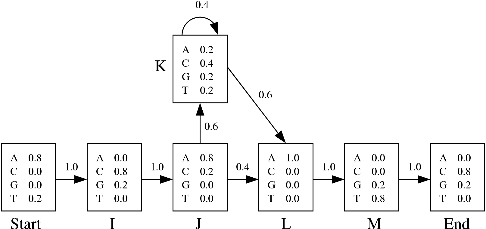
Figure 3.7: Basic HMM excerpted from the sequence analyst's bible[6]

Consider the basic output of a HMM profile building algorithm drawn in Figure 3.7.

Source

It can be translated into the following GenRGenS input file:

Figure 3.8: A Markovian description file for the $1$q$31.1$ area of the first human chromosome

Semantics

In 1, we choose a Markovian random generation.

In 2, an order of $1$ is defined for the master model.

In 3, we choose to manipulate words as symbols.

Part 4 is a definition for the frequencies of the master Markovian model. For instance, the probability of choosing L as the next hidden state while in state J is $p_{JL}=\frac{40}{100}$.
Remark: The word START is a keyword and cannot be used as an identifier.

Part 5 contains the different emission frequencies, converted from probabilities to integers.

Command-line options and additional tools

Markov-specific option: Dead-Ends tolerance

Inside some markovian models, it is theoreticaly possible that some states may be dead-ends, the frequencies of all candidate symbols summing to 0 in this context. It is then impossible to emit an extra symbol. That is why GenRGenS always checks weither each reachable state can be exited. The default behaviour of GenRGenS is to refuse to generate sequences in such a case, as the generated sequences are supposed to be of the size provided by the user, and it is senseless to keep on generating letters when a dead-end is encountered. However, this phenomenon may be intentional, in order for instance to end the generation with a specific word (perhaps a STOP codon...) if total control over the size can be neglected.

Markovian specific command line option usage:

java -cp . GenRGenS.GenRGenS -size n -nb k -m [T$\mid$F] MarkovianGGDFile

• -m [T$\mid$F]: Toggles rejection of models with dead-ends on (T) and off (F). Notice that disabling the rejection may result in shorter sequences than that specified by mean of the size parameter. Defaults to -m T.

BuildMarkov: Automatic construction of MARKOV description files

Tool description

This small software is dedicated to the automatic construction of MARKOV description files from a sequence. It scans the sequence(s) provided through the command line and evaluates the probabilities of transitions from and to each markov states.

Usage

After decompression of the GenRGenS archive, move to GenRGenSDir and open a shell to invoke the Java virtual machine through the following command:

java -cp . GenRGenS.markov.BuildMarkov [options] InputFiles

where:

-

InputFiles is a set of paths aiming at sequences that will be used for Markov model construction. Required(At Least one).

The following parameters/options can also be specified :

• -d OutputFile: Outputs the description file to the file OutputFile.
• -p $n$: Defines the number of phases in the markov model. $n$ must be $>0$. $n=1$ means that the model will be homogenous. Defaults to $n$=1.
• -o $k$: Defines the order of the markov model. $k$ must be $\ge0$. $k=0$ means that the model will be a bernoulli model. Defaults to $n$=0.
• -v $1$: Verbose mode, show the progress of the construction(useful for large files).

Input files

The input files can be flat files, that are text files containing a raw sequence, or FASTA formatted files, that are an alternation of title lines and sequences, and usually look like the figure below.

Figure 3.9: A typical FASTA formatted file, containing several sequences.

Remark1: Inside a sequence definition, both for FASTA and flat files, BuildMarkov ignores the spaces, tabulations and carriage returns so that the sequence can be indented in a user-friendly way.
Remark2: When several sequences are found inside a FASTA file, they are considered as different sequences and processed to build the Markov model. If the FASTA file contains a sequence split into contigs, thus needing to be concatenated, then a preprocessing of the file is required to remove the title lines before it can be passed as an argument to BuildMarkov.